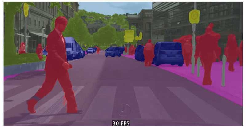
Image segmentation is one of the fundamentals tasks in computer vision alongside
with object recognition and detection. In semantic segmentation, the goal is to
classify each pixel of the image in a specific category. The difference from
image classification is that we do not classify the whole image in one class but
each individual pixel. So, we have a set of predefined categories and we want to
assign a label in each pixel of the image. And we do this assignment based on
the context of the different objects in the image.

ICNet for Real-Time Semantic Segmentation on High-Resolution Images
We can see a real-world example in the above image. Each pixel of the image has
been assigned to a specific label and represented by a different color. Red for
people, blue for cars, green for trees etc.
It is important to mention that semantic segmentation is different from instance
segmentation in which we distinguish labels for instances of the same class. In
that case, the people will all had a different color.
But we do we fraking care? (by the way, if you don’t know what frak means, go
binge watch Battlestar Galactica. It’s awesome). Why we need this high-detailed
processing?
It turns out that semantic segmentation has many different applications. You can
guess the first from the above image. Self-driving cars. Self-driving cars need
to know what they see. And they need to know everything. Every damn pixel.
Another popular use is of course in robotics( industrial or not). I can’t list
many more. Geosensing, agriculture, medical image diagnostics, facial
segmentation, fashion.
If you are convinced, let’s see how we can approach the task. It is not that
difficult to figure out.
Deep Learning
It is no secret that deep neural networks revolutionize computer vision and
especially image classification. From 2012 to today, it surpasses its
predecessors by a big margin. It is now a fact that computers are better in
image classification than humans. Inevitably then, we used the same techniques
for semantic segmentation too. And did they work?
Of course, they did. Convolutional Neural Networks are now the standard in the
industry for these kinds of problems. I am not going to bore you with a historic
flashback of all the architectures in the field. Instead, I will present to you
the state of the art, as it is appearing today .
But first let’s define our problem more specifically:
-
Each pixel of the image must be assigned to a class and colorized
accordingly -
The input and the output image should have exactly the same size
-
Each pixel on the input must correspond to a pixel in the exact same
location on the output -
We need pixel-level accuracy to distinguish between different classes.
Taken these into consideration, let’s proceed to the architecture:
Fully Convolutional Network (FCN)
Fully Convolutional networks consist of only convolutional and pooling layers,
without the need fully connected. The original approach was to use a stack of
same-sized convolutional layers to map the input image to the output one.

Stanford University School of Engineering
As you may imagine it produced quite good results, but it was extremely
computationally expensive. The thing was that they couldn’t use any downsampling
or pooling layers as it will mess up the location of the instances. And to
maintain the image resolution, they need to add many layers to learn both
low-level and high-level features. Thus, it ended being quite inefficient.
To solve this problem, they proposed an encoder-decoder architecture. The
encoder is a typical convolutional network such as AlexNet or ResNet[https://towardsdatascience.com/an-overview-of-resnet-and-its-variants-5281e2f56035] and the
decoder consists of deconvolutional (although I don’t like the term) and
up-sampling layers. The goal of downsampling steps is to capture
semantic/contextual information while the goal of upsampling is to recover
spatial information.

Stanford University School of Engineering
That way, they managed to reduce significantly the time and space complexity.
But also, the final result. Because the encoder reduces the image resolution,
the segmentation lacks well-defined edges, meaning that the boundaries between
the images are not clearly defined.
To the rescue: Skips Connections.
Skip connections bypass layers and transfer the information intact to the next
layers. In our case, we use them to pass the information from early layers of
the encoder to the decoder, bypassing the downsampling layers. And indeed, this
helped improve the details of the segmentation with much more accurate shapes
and edges.
UNet
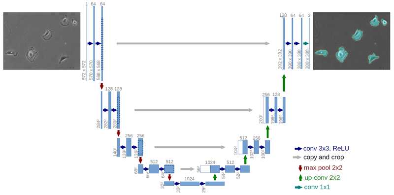
Based on the whole encoder-decoder and skip connection concept, the idea of
Fully Convolutional Network expanded to U-net. U-net introduces symmetry in
the FCN by increasing the size of the decoder to match the encoder and replaces
the sum operation in skip connections with a concatenation.
Due to the symmetry, we can transfer a lot more information from the
downsampling layers to the upsampling ones (as there are more features maps now
), improving that way the resolution of the final output.

https://datascience.stackexchange.com
U-nets have originally developed for biomedical image segmentation, but they
also used in a wide of different applications with many variations such as the
addition of fully connected layers or residual blocks.
To fully grasp the U-net idea, let’s write some code to realize how dead-simple
it is. We are going to use python and keras framework to simplify thing even
more.
def unet(pretrained_weights = None,input_size = (256,256,1)):
inputs = Input(input_size)
conv1 = Conv2D(64, 3, activation = 'relu', padding = 'same', kernel_initializer = 'he_normal')(inputs)
conv1 = Conv2D(64, 3, activation = 'relu', padding = 'same', kernel_initializer = 'he_normal')(conv1)
pool1 = MaxPooling2D(pool_size=(2, 2))(conv1)
conv2 = Conv2D(128, 3, activation = 'relu', padding = 'same', kernel_initializer = 'he_normal')(pool1)
conv2 = Conv2D(128, 3, activation = 'relu', padding = 'same', kernel_initializer = 'he_normal')(conv2)
pool2 = MaxPooling2D(pool_size=(2, 2))(conv2)
conv3 = Conv2D(256, 3, activation = 'relu', padding = 'same', kernel_initializer = 'he_normal')(pool2)
conv3 = Conv2D(256, 3, activation = 'relu', padding = 'same', kernel_initializer = 'he_normal')(conv3)
pool3 = MaxPooling2D(pool_size=(2, 2))(conv3)
conv4 = Conv2D(512, 3, activation = 'relu', padding = 'same', kernel_initializer = 'he_normal')(pool3)
conv4 = Conv2D(512, 3, activation = 'relu', padding = 'same', kernel_initializer = 'he_normal')(conv4)
drop4 = Dropout(0.5)(conv4)
pool4 = MaxPooling2D(pool_size=(2, 2))(drop4)
conv5 = Conv2D(1024, 3, activation = 'relu', padding = 'same', kernel_initializer = 'he_normal')(pool4)
conv5 = Conv2D(1024, 3, activation = 'relu', padding = 'same', kernel_initializer = 'he_normal')(conv5)
drop5 = Dropout(0.5)(conv5)
up6 = Conv2D(512, 2, activation = 'relu', padding = 'same', kernel_initializer = 'he_normal')(UpSampling2D(size = (2,2))(drop5))
merge6 = concatenate([drop4,up6], axis = 3)
conv6 = Conv2D(512, 3, activation = 'relu', padding = 'same', kernel_initializer = 'he_normal')(merge6)
conv6 = Conv2D(512, 3, activation = 'relu', padding = 'same', kernel_initializer = 'he_normal')(conv6)
up7 = Conv2D(256, 2, activation = 'relu', padding = 'same', kernel_initializer = 'he_normal')(UpSampling2D(size = (2,2))(conv6))
merge7 = concatenate([conv3,up7], axis = 3)
conv7 = Conv2D(256, 3, activation = 'relu', padding = 'same', kernel_initializer = 'he_normal')(merge7)
conv7 = Conv2D(256, 3, activation = 'relu', padding = 'same', kernel_initializer = 'he_normal')(conv7)
up8 = Conv2D(128, 2, activation = 'relu', padding = 'same', kernel_initializer = 'he_normal')(UpSampling2D(size = (2,2))(conv7))
merge8 = concatenate([conv2,up8], axis = 3)
conv8 = Conv2D(128, 3, activation = 'relu', padding = 'same', kernel_initializer = 'he_normal')(merge8)
conv8 = Conv2D(128, 3, activation = 'relu', padding = 'same', kernel_initializer = 'he_normal')(conv8)
up9 = Conv2D(64, 2, activation = 'relu', padding = 'same', kernel_initializer = 'he_normal')(UpSampling2D(size = (2,2))(conv8))
merge9 = concatenate([conv1,up9], axis = 3)
conv9 = Conv2D(64, 3, activation = 'relu', padding = 'same', kernel_initializer = 'he_normal')(merge9)
conv9 = Conv2D(64, 3, activation = 'relu', padding = 'same', kernel_initializer = 'he_normal')(conv9)
conv9 = Conv2D(2, 3, activation = 'relu', padding = 'same', kernel_initializer = 'he_normal')(conv9)
conv10 = Conv2D(1, 1, activation = 'sigmoid')(conv9)
model = Model(input = inputs, output = conv10)
model.compile(optimizer = Adam(lr = 1e-4), loss = 'binary_crossentropy', metrics = ['accuracy'])
if(pretrained_weights):
model.load_weights(pretrained_weights)
return model
Do you think I am kidding? That’s it. A bunch of convolutional, pooling and
upsampling layers stacked together and a few concatenations to implement the
skip connections. Dead-simple or what?
Of course, we still need a lot of work to do like preprocess our input data,
augment them and more importantly find them. What I mean is that gathering
ground-images for our training is not an easy task at all. Just think that for
every input image, we want its segmentation to find the error between them. And
how can we construct the ground truth segmentations? By hand? That’s a possible
way to do it. By a well- crafted script? Maybe. One thing is certain. It is not
easy.
Finally, I would like to mention that there are other pretty clever ways to
perform semantic segmentation but most of them are built upon the FCN and U-Net.
Some of them are:
For further exploration of the depths of Semantic Segmentation with Deep Learning, there is no better way
than the Advanced Computer Vision with TensorFlow course by DeepLearning.ai.
Semantic segmentation is a very active field of research due to its high
importance and emergency in real-world applications, so we expect to see a lot
more papers over the next years. The combination of computer vision and deep
learning is highly exciting and has given us tremendous progress in complicated
tasks. Do you think that Tesla autonomous cars would have driven 1 billion
miles by today without Deep Learning? I personally don’t think so. Let’s see
what the future holds…
* Disclosure: Please note that some of the links above might be affiliate links, and at no additional cost to you, we will earn a commission if you decide to make a purchase after clicking through.


