A neural network is an algorithm whose design was inspired by the functioning of the human brain. It tries to emulate the basic functions of the brain.
Due to the intentional design of ANNs as conceptual model of human brain let’s first understand how biological neurons work. Later we can extrapolate that idea into mathematical models.
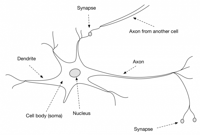
The below diagram is a model of the biological neuron

It consists of three primary parts, viz., the dendrites, soma, and the axon.
Dendrites are the receiver of the signals for the neuron. The dendrites collect the signal and pass it to soma, which is the main cell body.
Axon is the transmitter of the signal for the neuron. When a neuron fires it transmits its stimulus through the axon.
The dendrites of one neuron are connected to the axons of other neurons. Synapses are the connecting junction between axons and dendrites.
A neuron uses dendrites to collect inputs from other neurons, adds all the inputs, and if the resulting sum is greater than a threshold, it fires.
A neuron by itself is good for nothing. However, when we have lots of neurons connected, they are stronger and can do magic. In our brain, there are billions of connections like that to process and transmit information.
In our brain there are billions of interconnected neurons that enables us to sense, to think, and to take action.
ARTIFICIAL NEURON:
The artificial neuron is illustrated below

Here the inputs are equivalent to the dendrites of the biological neuron, the activation function is analogous to the soma and the output is analogous to the axons.
The artificial neuron will have inputs and each of the inputs will have weights associated with it. For now just know that weights are randomly initialized.
The weights here denotes that how important a particular node is. The inputs multiplied with the weights(weighted sum) will be sent as an input to the neuron.

Here, i is the index and m is the number of inputs
Once the weighted sum is calculated, an activation function will be applied to it. An activation function basically squashes the input between 0 and 1.
The result of the activation function decides whether to fire a neuron or not.

φ is the activation function.
I have written an article explaining some of the commonly used activation function. You can read my article Introduction to Activation Functions to learn more about them.
McCULLOCH-PITTS NEURON:
This was one of the earliest and extremely simple artificial neuron proposed by McCulloch and Pitts in 1943.
The McCulloch-Pitts neuron takes binary input and produces a binary output.
The weight for the McCulloch-Pitts neuron is chosen based on the analysis of the problem. The weight can either be excitatory or inhibitory. If the weight is positive, i.e., 1, then it is excitatory or if the weight is negative, i.e., -1 then it is inhibitory.
There is a threshold for each neuron, if the net input is higher than the threshold value, then that neuron fires.
Let’s see an example of how to implement logical AND gate using M-P neuron.
The following is the truth table for logic AND gate.
| X1 | X2 | Y |
| 0 | 0 | 0 |
| 0 | 1 | 0 |
| 1 | 0 | 0 |
| 1 | 1 | 1 |
Let’s assume the weights w1 = w2 = 1

For the inputs,
(0,0), y = w1*x1 + w2*x2 = (1×0) + (1×0) = 0
(0,1), y = w1*x1 + w2*x2 = (1×0) + (1×1) = 1
(1,0), y = w1*x1 + w2*x2 = (1×1) + (1×0) = 1
(1,1), y = w1*x1 + w2*x2 = (1×1) + (1×1) = 2
Now, we have to set the threshold value for which the neuron has to fire. Based on these calculated net input values the threshold is set.
For an AND gate the output is true only if both the inputs are true.
So, if we set the threshold value as 2, the neuron fires only if both the inputs are true.
Now let’s implement McCulloch-Pitts neuron using python
|
1 2 3 4 5 6 7 8 9 10 11 12 13 14 15 16 17 18 19 20 21 22 23 24
|
import pandas as pd import numpy as np
def threshold(x): return 1 if x >= 2 else 0
def fire(data, weights, output): for x in data: weighted_sum = np.inner(x, weights) output.append(threshold(weighted_sum))
data = [[0,0], [0,1], [1,0], [1,1]]
weights = [1, 1] output = []
fire(data, weights, output)
t = pd.DataFrame(index=None) t[‘X1’] = [0, 0, 1, 1] t[‘x2’] = [0, 1, 0, 1] t[‘y’] = pd.Series(output)
print(t) |
|
|
OUTPUT: X1 x2 y 0 0 0 0 1 0 1 0 0 1 1 1 |
SUMMARY:
In this post, we briefly looked at one of the earliest artificial neuron called McCulloch-Pitts neuron. We discussed the workings of the M-P neuron and also see how it is analogous to the human brain.
The problem with M-P neuron is that there is no real learning involved. We obtain the weight and the threshold value manually by performing the analysis of the problem. This completely contrasts the idea of learning from experience.
In the next part, we will see the perceptron algorithm, which is an improvement from the M-P neuron, which can learn the weights over time.
To get the complete code visit this Github Repo.


