Introduction to Decision Trees

Decision trees are one of the most powerful and widely used supervised models that can either perform regression or classification. In this tutorial, we’ll concentrate only on the classification setting.

A decision tree consists of rules that we use to formulate a decision on the prediction of a data point. Basically, it’s a sequence of simple if/else rulings.

We can visualize the decision tree as a structure based on a sequence of decision processes on which a different outcome can be expected.

Source: Machine learning Quick ReferenceBeginning at the root node of a tree, the decision node represents the basis on which a decision is made with each possible outcome resulting in a branch. Each branch represents how a choice may lead either to a decision nodes or to a leaf node, and each terminal represents the outcome.

Constructing a decision tree:

It’s important to understand how to build a decision tree. So let’s take a simple example and build a decision tree by hand.

Suppose the following training dataset is given. We need to determine the class label using the four features age, income, student, credit_rating.

There are three different ways to make a split in the decision tree.

Information Gain and Entropy
Gini index
Gain ratio

In this tutorial, we’ll see how to identify which feature to split upon based on entropy and information gain.

ENTROPY AND INFORMATION GAIN:

Entropy came from information theory and measures how randomly the values of the attributes are distributed. It is a measure of randomness or uncertainty.

Entropy is defined as follows

\mathrm{E}=\sum_{i=0}^{n}-\mathrm{p}_{\mathrm{i}} \log _{\mathrm{2}} \mathrm{p}_{\mathrm{i}}

Suppose if we toss an unbiassed fair coin with a 50% chance of heads and 50% chance of tails, then the entropy is as follows

E=-0.5 * \log _{2}(0.5)-0.5 * \log _{2}(0.5)=0.5+0.5=1

On the other hand, if we have a biased coin, with a 25% chance of heads and a 75% chance of tails, then the entropy is equal to

E=-0.25 * \log _{2}(0.25)-0.75 * \log _{2}(0.75)=0.81127812445

The decision tree tries to find the splits that reduce entropy and increase homogeneity within the groups.

Now we want to determine which attribute is most useful. Information gain tells us how important an attribute is.

To describe information gain, we first need to calculate the entropy of the distribution of labels. We have nine tuples of class ‘yes’ and five tuples of class ‘no’.The entropy belonging to the initial distribution is as follows.

E(D)=-\frac{9}{14} \log _{2}\left(\frac{9}{14}\right)-\frac{5}{14} \log _{2}\left(\frac{5}{14}\right)=0.940

The formula for the information gain is given as follow

Information gain = Entropy (parent) – Weighted Average * Entropy (children)

Now, we need to compute entropy for each attribute and choose the attribute with the highest information gain as the root node.

Let’s calculate the entropy for the age attribute.

\begin{aligned}E(Age) &=\frac{5}{14} \times\left(-\frac{2}{5} \log _{2} \frac{2}{5}-\frac{3}{5} \log _{2} \frac{3}{5}\right) \\&+\frac{4}{14} \times\left(-\frac{4}{4} \log _{2} \frac{4}{4}\right) \\&+\frac{5}{14} \times\left(-\frac{3}{5} \log _{2} \frac{3}{5}-\frac{2}{5} \log _{2} \frac{2}{5}\right) \\&=0.694 \end{aligned}

Hence the gain in information for partition at age is

\text {InfoGain }(a g e)=E(D)-E(age)=0.940-0.694=0.246

Similarly, the information gain for the remaining attributes are

InfoGain(income) = 0.029

InfoGain(student) = 0.151

InfoGain(credit_rating) = 0.048

Here the attribute age has the highest information gain of 0.246, so we can select age as the splitting attribute.

The root node is labeled as age, and the branches are grown for each of the values of the attribute.

The attribute age can take three values low, medium, and high.

Since the instances falling in the partition middle_aged all belong to the same class, we’ll make it a leaf node labeled ‘yes.’

Now again, we have to repeat the process recursively to form a decision tree at each partition.

The fully grown decision tree is given below.

STOPPING CRITERIA:

The decision tree grows until each leaf nodes are pure, i.e., all the points in the leaf node belong to a single class. Such trees can lead to overfitting and less accurate on unseen data.

As the depth of the tree increases, the accuracy in the training data may increase, but it will not generalize for unseen data.

So we need to balance the trade-off between the maximum depth of the tree and the accuracy.

Some of the commonly used stopping criteria are

No attribute satisfies a minimum information gain threshold
The tree has grown to a maximum depth
Number of samples in the subtree is less than the threshold

Now let’s implement Decision Tree using scikit-learn

import numpy as np from sklearn.tree import DecisionTreeClassifier from sklearn.datasets import load_iris from sklearn.model_selection import train_test_split from sklearn.metrics import accuracy_score np.random.seed(2020) data = load_iris() X = data.data y = data.target X_train, X_test, y_train, y_test = train_test_split(X, y, test_size=0.3) clf = DecisionTreeClassifier() clf.fit(X_train, y_train) y_pred = clf.predict(X_test) print(accuracy_score(y_test, y_pred))

import numpy as np

from sklearn.tree import DecisionTreeClassifier

from sklearn.datasets import load_iris

from sklearn.model_selection import train_test_split

from sklearn.metrics import accuracy_score

np.random.seed(2020)

data = load_iris()

X = data.data

y = data.target

X_train, X_test, y_train, y_test = train_test_split(X, y, test_size=0.3)

clf = DecisionTreeClassifier()

clf.fit(X_train, y_train)

y_pred = clf.predict(X_test)

print(accuracy_score(y_test, y_pred))

CONCLUSION:

A decision tree is a supervised machine learning algorithm that can either perform classification or regression. The decision tree is built recursively in a top-down manner.

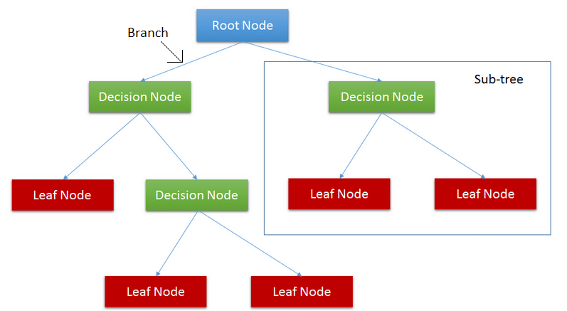
Various components of the tree are

ROOT NODE: The root node represents the entire sample.

DECISION NODE: Nodes are where a decision is taken.

BRANCH: Branch represents how a choice may lead to a decision.

LEAF NODE: The final node in a decision tree. Each leaf node holds a class label.

The code for this tutorial can be found in this Github Repo.

Source link