Brain MRI Segmentation | Python | Tensorflow | Keras

In this article we’ll see how to perform Brain tumor segmentation from MRI images. We’ll try different architectures which are popular for image segmentation problems.

Let’s start by defining what our business problem is.

Business Problem:

A brain tumor is an abnormal mass of tissue in which cells grow and multiply abruptly, which remains unchecked by the mechanisms that control normal cells.

Brain tumors are classified into benign tumors or low grade (grade I or II ) and malignant or high grade (grade III and IV).Benign tumors are non-cancerous and are considered to be non-progressive, their growth is relatively slow and limited.

However, malignant tumors are cancerous and grow rapidly with undefined boundaries. So, early detection of brain tumors is very crucial for proper treatment and saving of human life.

Problem Statement:

Dataset:

The dataset is downloaded from Kaggle.

This dataset contains brain MRI images together with manual FLAIR abnormality segmentation masks.

The images were obtained from The Cancer Imaging Archive (TCIA). They correspond to 110 patients included in The Cancer Genome Atlas (TCGA) lower-grade glioma collection with at least fluid-attenuated inversion recovery (FLAIR) sequence and genomic cluster data available.

Tumor genomic clusters and patient data is provided in data.csv file. The images are in tif format

Exploratory Analysis and Pre-Processing:

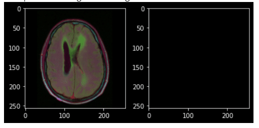
The following is a sample image and its corresponding mask from our data set. 

Let’s print a brain image which has tumor along with its mask.

Now Let’s check the distribution of tumorous and non-tumor images in the data set.

Here 1 indicates tumor and 0 indicates no tumor. We have a total of  2556 non-tumorous and 1373 tumorous images.

As a pre-processing step we’ll crop the part of the image which contains only the brain. Before cropping the image we have to deal with one major problem that is low contrast.

A common problem with MRI images is that they often suffer from low contrast. So, enhancing the contrast of the image will  greatly improve the performance of the models.

For instance, take a look at the following image from our data set.

With the naked eye we cannot see anything. It’s completely black. Let’s try enhancing the contrast of this image.

There are two common ways to enhance the contrast.

1. Histogram Equalization and
2. Contrast Limited Adaptive Histogram Equalization(CLAHE)

First we’ll try Histogram Equalization. We can use OpenCV’s equalizeHist()

The following is the histogram equalized image.

Now let’s apply CLAHE. We’ll use OpenCV’s createCLAHE() 

The following is the image after applying CLAHE

The above image depicts the process of contrast enhancing and cropping for a single image. Similarly we’ll do this for all the images in the data set.

The following code will perform the pre-processing step and save the cropped images and its masks.

Evaluation Metrics:

Before proceeding to the modelling part we need to define our evaluation metrics.

The most popular metrics for image segmentation problems are Dice coefficient and Intersection Over Union(IOU).

IOU:

IoU is the area of overlap between the predicted segmentation and the ground truth divided by the area of union between the predicted segmentation and the ground truth.

IOU = \frac{\mathrm{TP}}{\mathrm{TP}+\mathrm{FN}+\mathrm{FP}}

Dice Coefficient:

The Dice Coefficient is 2 * the Area of Overlap divided by the total number of pixels in both images.

Dice Coefficient = \frac{2 T P}{2 T P+F N+F P}

1 – Dice Coefficient will yield us the dice loss. Conversely, people also calculate dice loss as -(dice coefficient). We can choose either one.

However, the range of the dice loss differs based on how we calculate it. If we calculate dice loss as 1-dice_coeff then the range will be [0,1] and if we calculate the loss as -(dice_coeff) then the range will be [-1, 0].

If you want to learn more about IOU and Dice Coefficient you might want to read this excellent article by  Ekin Tiu.

Models:

I have totally trained three models. They are

1. Fully Convolutional Network(FCN32)
2. U-NET and
3. ResUNet

The results of the models are below.

As you can see from the above results, the ResUNet model performs best compared to other models.

However, if you take a look at the IOU values it is near 1 which is almost perfect. This could be because the non-tumor area is large when compared to the tumorous one.

So to confirm that the high Test IOU is not because of that let’s calculate the IOU values for the tumor and non-tumour images separately.

We’ll first divide our test data into two separate data sets. One with tumorous images and the other with non-tumorous images.

Once we have divided the data set we can load our ResUnet model and make the predictions and get the scores for the two data sets separately.

The following are the results separately on the tumorous and non-tumorous images.

The numbers looks Okay. So, we can conclude that the score is not high because of the bias towards the non-tumorous images which has relatively large area when compared to tumorous images.

The following are the sample results of the ResUNet model.

The results are looking good. The image on the left is the input image. The middle one is the ground truth and the image which is on the right is our model’s(ResUNet) prediction.

To get the complete code for this article visit this Github Repo.

References: