Explainable AI (XAI): A survey of recents methods, applications and frameworks

Deep learning applications have drawn a lot of attention since they have surpassed humans in many tasks such as image and speech recognition, and recommendation systems. However, these applications lack explainability and reliability.

Deep learning models are usually considered as black boxes that are hard to understand while their underlying mechanism is complex.

They do not justify their decisions and predictions and humans cannot trust them. On the other hand, artificial intelligence algorithms make errors that could be fatal depending on the application.

More specifically, an error in a computer vision system of an autonomous car could lead to a crash, while in the medical area, human lives are depending on these decisions.

Most machine learning models perform as black boxes.

To tackle the aforementioned issues, a plethora of methods have been developed. To this end, eXplainable Artificial Intelligence (XAI) has become a hot research topic in the machine learning community.

These methods aim to provide explanations about machine-deep learning models that are easily understandable by humans.

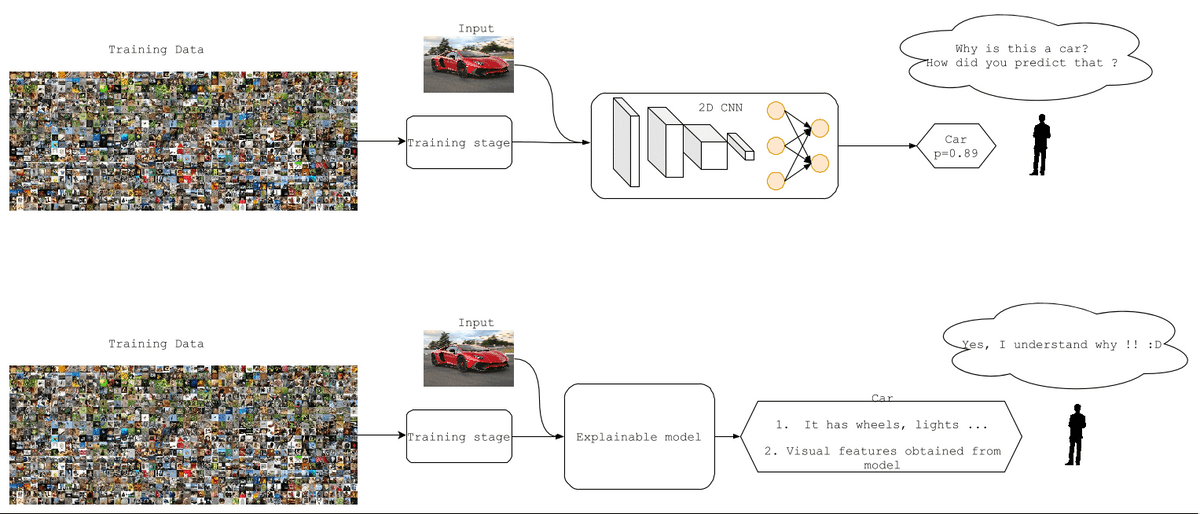
Comparison of a deep learning and an explainable model.

Categories of Interpretability

Interpretability defines how easily we can understand the cause of a decision that is produced from an algorithm.

The adopted categorization of interpretability methods is based on how explanation information is provided.

In this article, the following categories will be discussed:

Visual interpretability methods: visual explanations and plots
Textual explanations, given in text form
Mathematical or numerical explanations

Visual explanations

Visual explainable methods produce pictures or plots in order to provide information about the model’s decision.

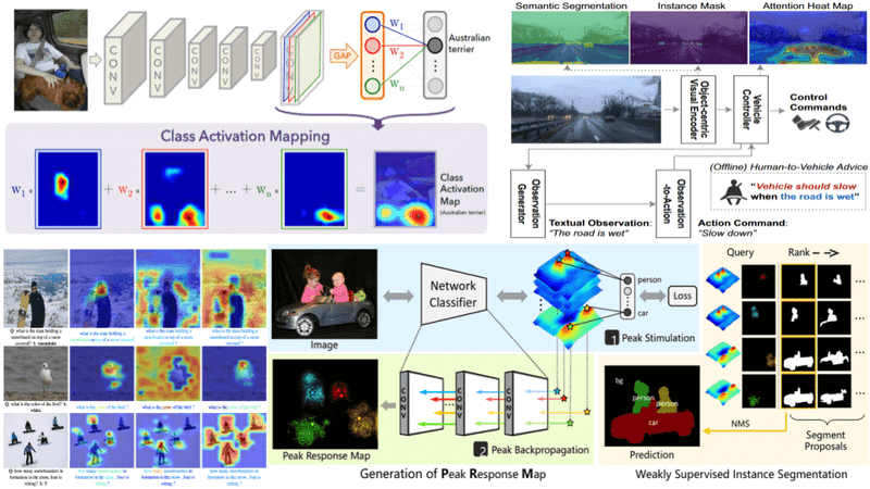
Most methods explain the decision of a model in the form of a saliency map by producing values to reflect the importance and contribution of input components to that decision.

These values can take the form of output probabilities or images like heatmaps. In addition, plot visualization methods produce scatter plots to explain decisions or visualize the data.

Class Activation Mapping (CAM)

One of the first and most popular saliency methods is Class Activation Mapping (CAM) [28]. CAM is able to localize the features of the CNN on the image that are responsible for the classification decision. More specifically, CAM uses a global average pooling layer after the convolutional layers and before the final fully connected layer.

Let $f_{k}(x,y)$

\mathbf{S}_{c} = \sum_{x,y}\sum_{k}w_{c}^{k}f_{k}(x,y)

Finally, the class activation map $M_c$

M_{c}(x,y) =\sum_{k}w_{c}^{k}f_{k}(x,y)

and shows directly the importance of the activation at spatial point (x,y) to classify it’s class $c$ .

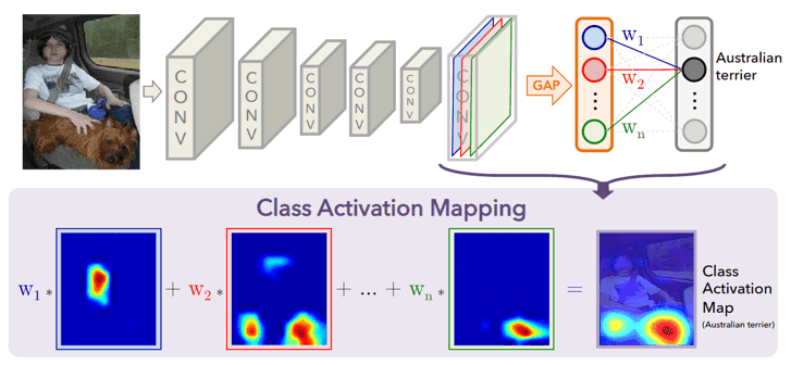
The predicted score is mapped to the last layer in order to generate the activation. The class-important regions are highlighted in CAM. Source: [28]

Gradient-weighted Class Activation Mapping (Grad-CAM)

Later on, Gradient-weighted Class Activation Mapping (Grad-CAM) was introduced. Grad-CAM [22] is an extended work based on CAM, which uses the gradients with respect to the target class $c$ that flows to the final convolutional layer. Grad-CAM produces a coarse localization map $\mathbf{L_{Grad-CAM}^{c}} \in \mathbb{R}^{v\times u}$

a_{k}^{c}= \frac{1}{Z} \sum_{i} \sum_{j} \frac{\partial y^{c}}{\partial A_{k}(i,j)}

The weighting factor $a_{k}^{c}$ Finally, the Grad-CAM heatmaps are produced using the forward propagation activations as:

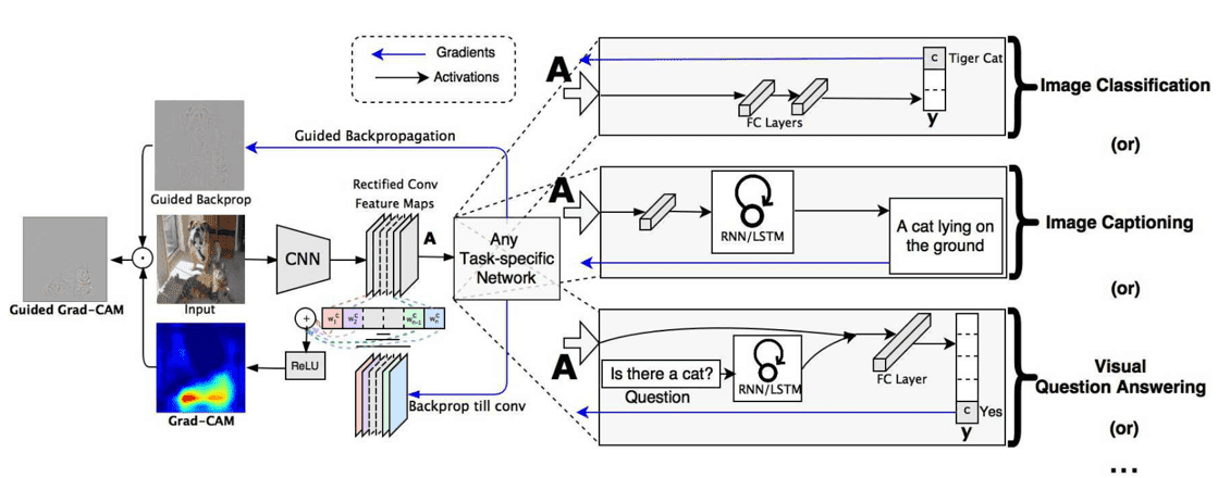
\mathbf{L_{Grad-CAM}^{c}}= ReLU(\sum_{k}a_{k}^{c}\mathbf{A_{k}})

Overview of Grad-CAM. Source: [22]

Layer-Wise Relevance Propagation (LRP)

Another visual explanation technique that has been adopted is Layer-Wise Relevance Propagation (LRP). LRP [23] is based on the decomposition of the decision and produces relevance scores between the activations $x(i)$ of neuron $i$ and its input, and finds the neuron’s importance scores $R^{l}(i)$ More specifically, the relevance scores $R^{l}(i)$

R^{l}(i) = \sum_{j}\frac{x(i)w(i,j)}{\sum_{i}x(i)w(i,j)}R^{l+1}(j)

where $w(i,j)$

The pixel-wise contributions to the classification are displayed as shown below:

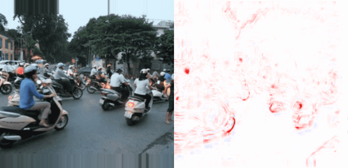
LRP visualization. Source: [23]

Subsequently, Peak Response Maps (PRM)

Subsequently, Peak Response Maps (PRM) were introduced for weakly supervised instance segmentation. PRM [29] finds the maximum class activations that specify the class scores in each image location. Then, these activations are back-propagated to the input image to generate the peak response maps. The peak’s locations

\mathbf{P_{c}} = \{(i_{1},j_{1}), …, (i_{N^{c}},j_{N^{c}})\}

where $N^{c}$

G^{c} (x,y)= \sum_{k=1}^{N^{c}} f(x-i_{k},y-j_{k})

where $x\in[0,H], y\in[0,W]$

{\delta}^{c} = \frac{1}{N^{c}}\frac{\partial L}{\partial \mathbf{s}^{c}} \mathbf{G}^{c}

where $L$ is the classification loss.

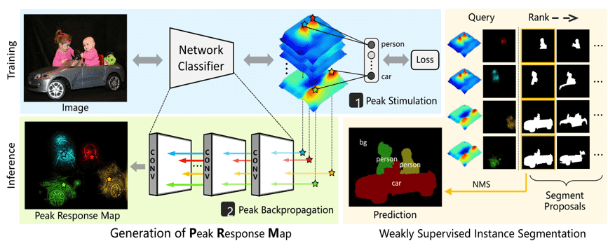
Peak Response Maps method. Source: [29]

CLass-Enhanced Attentive Response (CLEAR)

CLass-Enhanced Attentive Response (CLEAR) [11] is a similar approach that visualizes the decisions of a deep neural network using the activation values of the network. It used deconvolutions to obtain individual attention maps for each class. After the forward pass, we use deconvolutions to obtain the deconvolved output of layer $l$ with $K$ kernels as:

\mathbf{h}(l) = \sum_{k=1}^K z(k,l) * w(k,l)

where $\mathbf{z}(l)$ are the feature maps of the layer $l$ and $\mathbf{w}(l)$ are the kernel weights. The final response of layer $l$ is obtained from:

\mathbf{R}(l) = \mathbf{h}(1) \mathbf{h}(2)…. \mathbf{h}(l)

The individual attention maps $\mathbf{R(x’},c)$

\mathbf{R(x’},c) = \mathbf{h}(1) \mathbf{h}(2)…. \mathbf{h}(L)

Then, the dominant class attentive map $\mathbf{C(x’)}$

\mathbf{C(x’)} = {argmax}_c \mathbf{R(x’},c)

while the dominant response map $\mathbf{D_C(x’)}$

\mathbf{D}_c(\mathbf{x’}) = \mathbf{R(x’},c)

The dominant response map shows the attention at each location of the image, while the dominant class-map shows the most important class that was involved in the classification of the image.

Finally, the CLass-Enhanced Attentive Response (CLEAR) map is generated by overlaying the two aforementioned maps as:

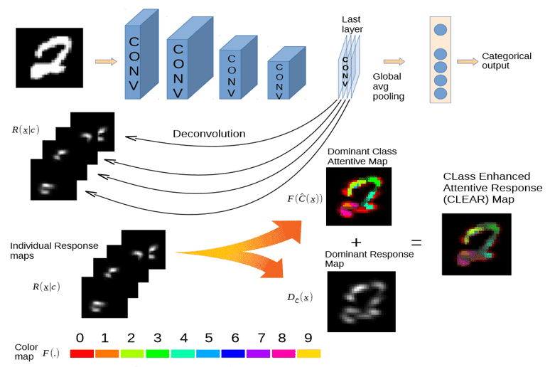
\textbf{M} = \mathbf{C(x’)}+ \mathbf{D}_c(\mathbf{x’}).

CLEAR method overview. Source: [11]

Visualization of features activations with Deconvolutional Networks

Zeiler et al.[27] tried to visualize the intermediate layers of convolutional neural networks and see what they learn. It was shown that convolutional layers store important information about the images as well as that deeper layers learn more complex patterns. In addition, de-convolutional neural networks were adopted in order to reconstruct the input images from feature maps in reverse order. This inverse operation creates an approximate image showing that CNNs have stored the most information of the image.

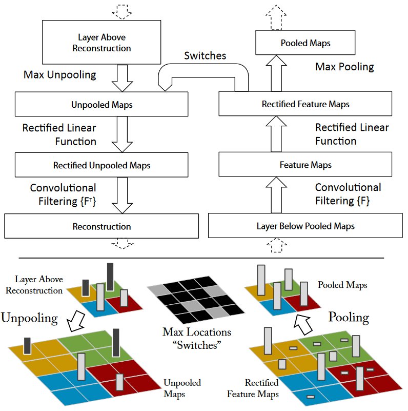
De-convolutional neural network. Source: [27]

DeepResolve

On the other hand, DeepResolve [12] method uses feature maps from intermediate layers and examines how the network combines those features to classify an input image. DeepResolve computes a class-specific image that is named as feature importance map (FIM):

\mathbf{H^{c}} = {argmax}_{\mathbf{H}}( S_{c}(\mathbf{H})-\lambda{||\mathbf{H}||}^{2}_{2})

where $c$ is the target class, $S_{c}$

\phi_{c}^{k} = \frac{1}{W} \sum_{i=1}(H^{k}(i))_c,

where $i$ is the index of the neuron and $k$ the index of the channel in a layer . This process is initialized randomly and is repeated $T$ times with different initial parameters to get several estimations of $\mathbf{H}_c^t, \mathbf{\Phi}_c^t$

IL_c^k = var(\phi_c^t)

and is used to obtain the overall neuron importance scores (ONIVs ) $\mathbf{\bar{\Phi}}_c$

The Class difference matrix is calculated as:

D_{C_i C_j} = \bar{\Phi}_{C_i} – \bar{\Phi}_{C_j}

between each pair of classes $C_i,C_j$

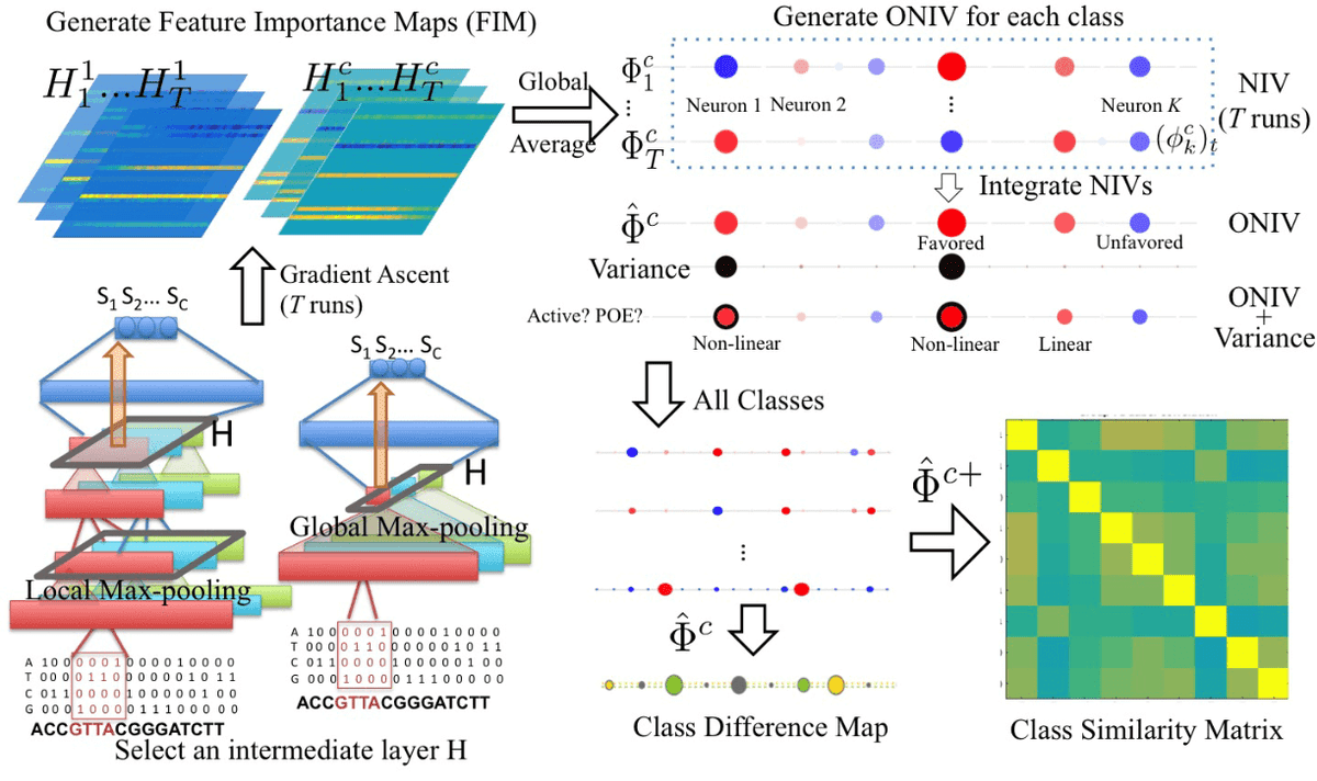
Illustration of DeepResolve’s working flow. Source: [12]

SCOUTER

A visual explanation method named SCOUTER [13] was recently introduced and is not based on feature maps and gradients to explain decisions. SCOUTER adopts a slot-attention classification layer instead of a fully connected layer.

The output features $\mathbf{F}$ (from a convolutional neural network) are transformed to a smaller dimension through another convolutional layer, while a position embedding layer models the spatial information. A self-attention mechanism is used to obtain the dot-product attention as :

\mathbf{A}^{(t)} = \sigma (Q(\mathbf{W}^{(t)})K(\mathbf{F})),

where $Q, K$

Then, the weighted feature map is calculated as :

\mathbf{U}^{(t)} = \mathbf{A}^{(t)}\mathbf{F}’^{(t)}

A recurrent GRU layer updates the slot weights as follows:

\mathbf{W}^{(t+1)} = GRU(\mathbf{U}^{(t)},\mathbf{W}^{(t)})

Each slot produces an interpretable confidence score $\mathbf{o}=(o_{1}, o_{2}, …, o_{n}$

\mathbf{o} = xSlot_{e}(\mathbf{F}) = e\cdot \mathbf{U}^{(t)}\mathbf{1_{c}},

where $e \in [-1,1]$

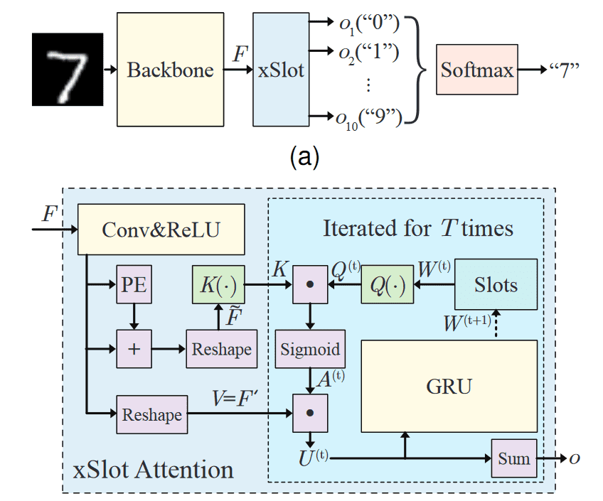
Illustration of Scouter. Source: [13]

Visual feedback

In [19], the authors proposed an interpretable method to identify relevant features for image classification. During training, the most important layers and filters for classification are identified, while in test time visual maps are generated to show the image locations that are responsible for this decision. More specifically, the class $j$ is predicted by the linear combination $\mathbf{w_{j}} \in \mathbb{R}^{m}$

\mathbf{W}^{*} = argmin_{\mathbf{W}} {||\mathbf{X}^{T}\mathbf{W} -\mathbf{ L}^{T} ||}^{2}_{F}

where $L$ are the ground-truth labels, to find the most relevant features of each class.

Visual explanations using relevant features. Source: [19]

At test time, the internal activations and the learned weights $\mathbf{W}$ are used to generate the decision after the forward pass of the test image $\mathbf{I}$ . Then, a class prediction is calculated as $\hat{y} = F(\mathbf{I})$

Plot visualization methods

In this section, we will describe methods that adopt scatter-plots or graph visualizations to generate explanations.

T-distributed stochastic neighbor embedding (t-SNE) is a scatter-plot method that projects high-dimensional data in two or three-dimensional spaces. t-SNE uses conditional probabilities to represent the distances between data points and find similarities. Finally, it uses a similar probability distribution over the points in the two or three-dimensional map and it minimizes the Kullback–Leibler divergence between these distributions.

Visualizing the Hidden Activity of Neural Networks with tSNE

In [20], the authors use t-SNE to visualize the activations of the neurons and the learned representations of the data. It is shown that these projections can provide valuable feedback about the relationships between neurons and classes.

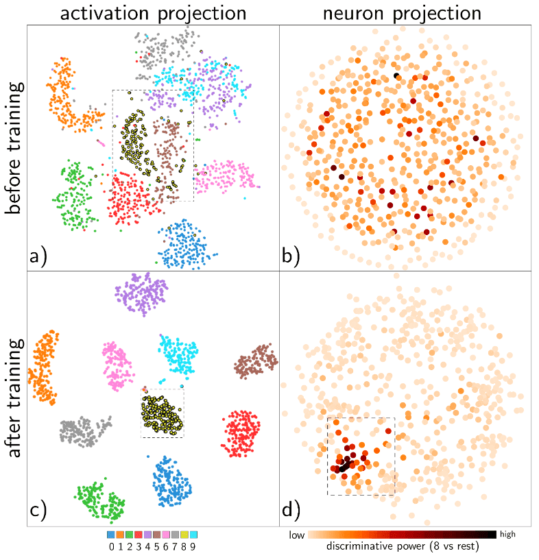
Visualization of hidden activity of neurons on MNIST dataset. Source: [20]

Explain features with PCA

In [3], Principal Component Analysis (PCA) was adopted to explain features from deep neural networks.

Given an input image of an image $r_{\theta} \in \mathbf{\Omega}$

\mathbf{F}^{L}(r_{\theta})=\mathbf{\hat{F}}^{L}(r_{\theta})-\frac{1}{\Theta}\sum_{t=1 }^{\Theta}\mathbf{\hat{F}}^{L}(r_{t})

we compute the eigenvectors by finding the eigenvalues of the covariance matrix:

\frac{1}{\Theta}\sum_{\theta =1}^{\Theta}(\mathbf{F}^{L}(\theta)){(\mathbf{F}^{L})(\theta)}^{T}

Then, the embeddings with the largest variance, i.e., the largest eigenvalues, are projected. In addition, the authors assume that the images can be decomposed into linear combinations of scene factors such as the view (position, rotation), colors or lightning and perform again the PCA dimensionality reduction on the decomposed features. Given parameters $\mathbf{\Theta} = \Theta_1, \Theta_2,…, \Theta_N$

\mathbf{F}_k^L(t) = \frac{|\Theta_k|}{|\Theta|}\sum_{\theta\in\Theta|\theta_k=t}\mathbf{F}^L(\theta)

In the figure below, image embeddings are projected with respect to different image factors.

Image embeddings projection. Source: [3]

TreeView

TreeView [25] is a method that tries to partition the feature space and into smaller subspaces where each subspace represents a specific factor. At first, the input data $\mathbf{X}$ is transformed into features $\mathbf{Y}$ . Subsequently, features $\mathbf{Y}$ are classified and transformed to label space $\mathbf{Z}$ . The aforementioned transformations are denoted as $T_1 : \mathbf{X} \rightarrow \mathbf{Y}$

We partition the feature space of $\mathbf{Y}$ into $K$ partitioned subspaces, which are constructed by clustering similar neurons according to their activations. Each cluster $i$ describes a specific factor $S_i$

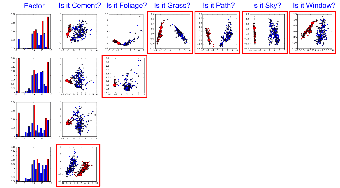
TreeView explanation. Source: [25]

Textual explanation methods

Some works have focused on textual interpretability. In general, textual explanation methods produce natural language-text to interpret the decisions.

Cell Activation Value

Cell Activation Values [8] is an explainability method for LSTMs. This method adopts character-level language to understand the long-term dependencies of LSTM modules. The input characters are projected into a lower-dimensional space. Subsequently, these vectors are fed to the LSTM at each timestep and projected to word sequences with fully connected layers. The activation values at each timestep model the next character in the sequence and are used to interpret the model.

Interpnet

Recently, Barratt et. al. [4] proposed a deep neural network, named Interpnet, that can be combined with a classification architecture and generate explanations. Let us consider a simple network as follows:

\mathbf{y} = softmax(\mathbf{W}_{1}relu(\mathbf{W}_{2}\mathbf{x}+\mathbf{b}_{2})+\mathbf{b}_{1})

and the internal activations $\mathbf{f}_1, \mathbf{f}_2, \mathbf{f}_3$

\mathbf{f}_1 = \mathbf{x}, \mathbf{f}_2 = relu(\mathbf{W}_{2}\mathbf{x}+\mathbf{b}_{2}), \mathbf{f}_3 = softmax(\mathbf{W}_{1}relu(\mathbf{W}_{2}\mathbf{x}+\mathbf{b}_{2})+\mathbf{b}_{1})

Interpnet uses the concatenated vector $\mathbf{r} =[\mathbf{f}_1; \mathbf{f}_2; \mathbf{f}_3]$

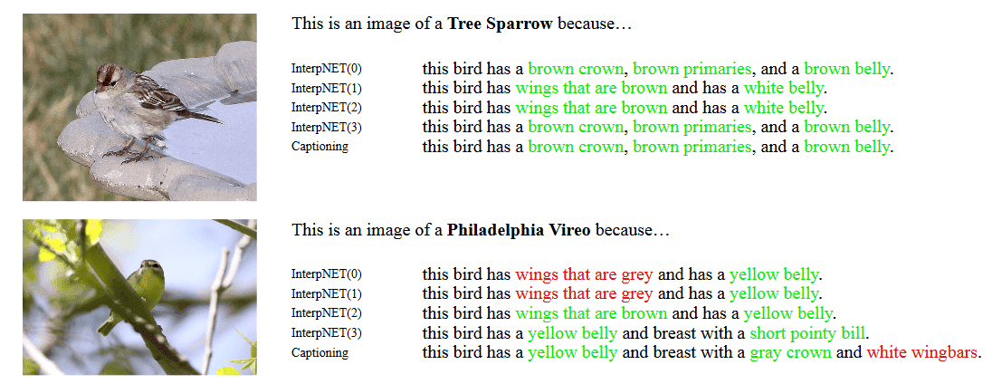
Interpnet generates explanations for the input images. Source:[4]

Visual Question Answering (VQA)

Here, the authors proposed a Visual Question Answering (VQA) [14] framework that jointly attends the image regions and the words of the question to generate the answer as depicted in Figure. At first, the words of the question $\mathbf{Q} = (\mathbf{q}_{1}, \mathbf{q}_{2}, …, \mathbf{q}_{T})$

\mathbf{q}_{t}^{h} = max(LSTM(conv(\mathbf{q}_{t:t+s}^{h})))

where $s$ is the receptive field of the 1D convolution layer.

A co-attention mechanism takes as input the image features $\mathbf{V}=(\mathbf{v_1},\mathbf{v_2},…,\mathbf{v_N})$

\mathbf{h}^w = tanh(\mathbf{W}_w(\mathbf{q}^{w}_{att} + \mathbf{v}^{w}_{att})

\mathbf{h}^p = tanh(\mathbf{W}_p[(\mathbf{q}^{p}_{att} + \mathbf{v}^{p}_{att}),\mathbf{h}^w]

\mathbf{h}^s = tanh(\mathbf{W}_s[(\mathbf{q}^{s}_{att} + \mathbf{v}^{s}_{att}),\mathbf{h}^p]

\mathbf{p} = softmax(\mathbf{W}_h\mathbf{h}^s)

where $\mathbf{W}_w, \mathbf{W}_p, \mathbf{W}_s, \mathbf{W}_h$

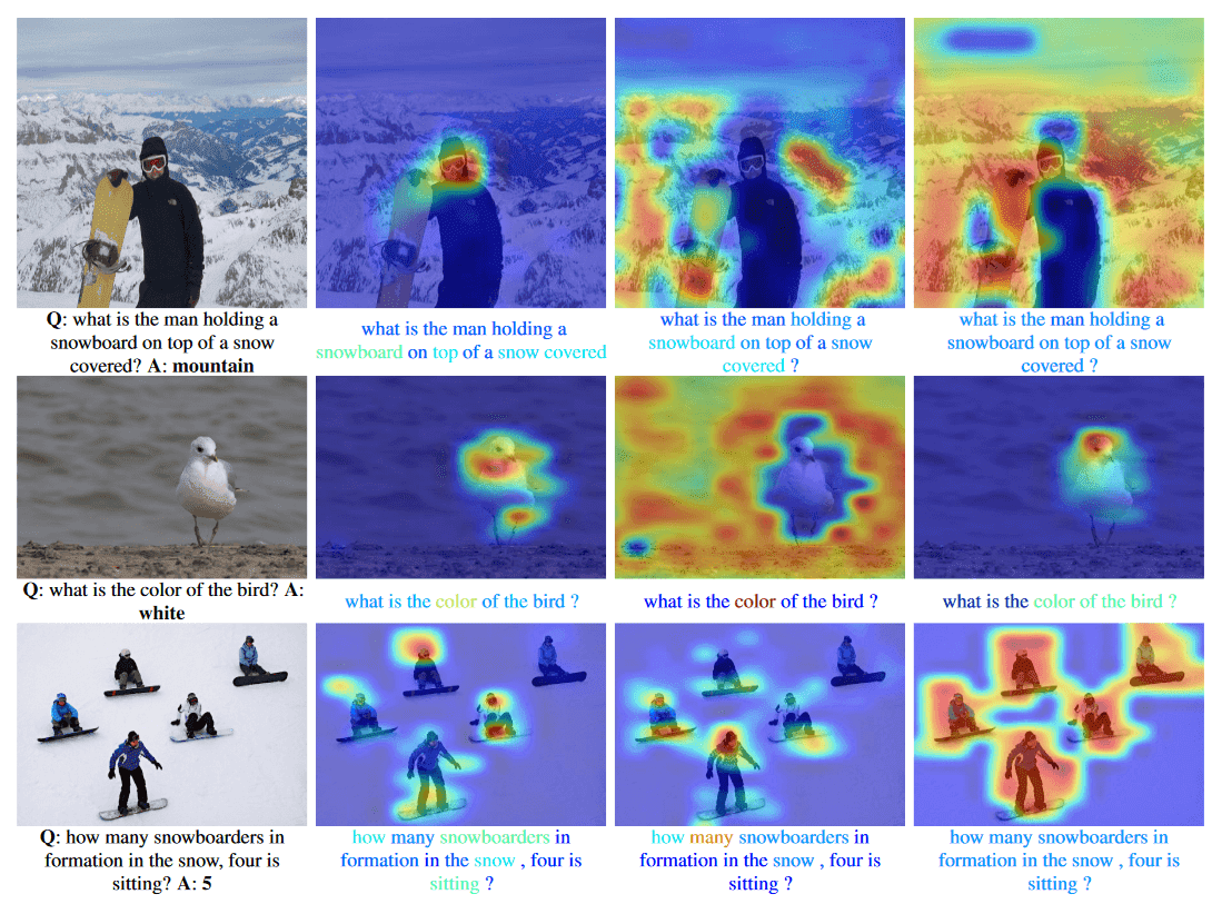
Example of questions and answers predicted word-level co-attention maps, phrase-level co-attention maps and question-level co-attention maps. Source: [4]

Semantic information to interpret Neural Networks

In [7], the authors employed semantic information to interpret deep neural networks (DNNs) for video captioning. A sample video-description pair has a video $\mathbf{x}$ with $n$ frames and $N_d$

a_i^t= \frac{exp(\mathbf{w}_a tanh(\mathbf{U}_a \mathbf{h}_{t-1}+\mathbf{T}_a \mathbf{v}_i +\mathbf{b}_a))}{ \sum_{j=1}^n exp(\mathbf{w}_a tanh(\mathbf{U}_a \mathbf{h}_{t-1}+\mathbf{T}_a \mathbf{v}_j +\mathbf{b}_a))}

$\mathbf{b}_a, \mathbf{T}_a, \mathbf{U}_a, \mathbf{w}_a$

\mathbf{p}_t = softmax(\mathbf{W}_p [\mathbf{h}_t, \phi_t (\mathbf{V}), \mathbf{y}_{t-1}] + \mathbf{b}_p)

The system uses descriptions of humans, denoted as $\mathbf{s}$ , that have information about the data. These descriptions are embedded in the network with a loss function defined as:

L_I(\mathbf{v},\mathbf{s}) = {||f(\frac{1}{n}\sum_{i=1}^n \mathbf{v}_i) – \mathbf{s}||_2^2}

and guide the learning process to learn interpretable features. This guides the neurons of the network to be associated with a specific topic and the whole network can be easily understandable by humans instead of being a black-box model.

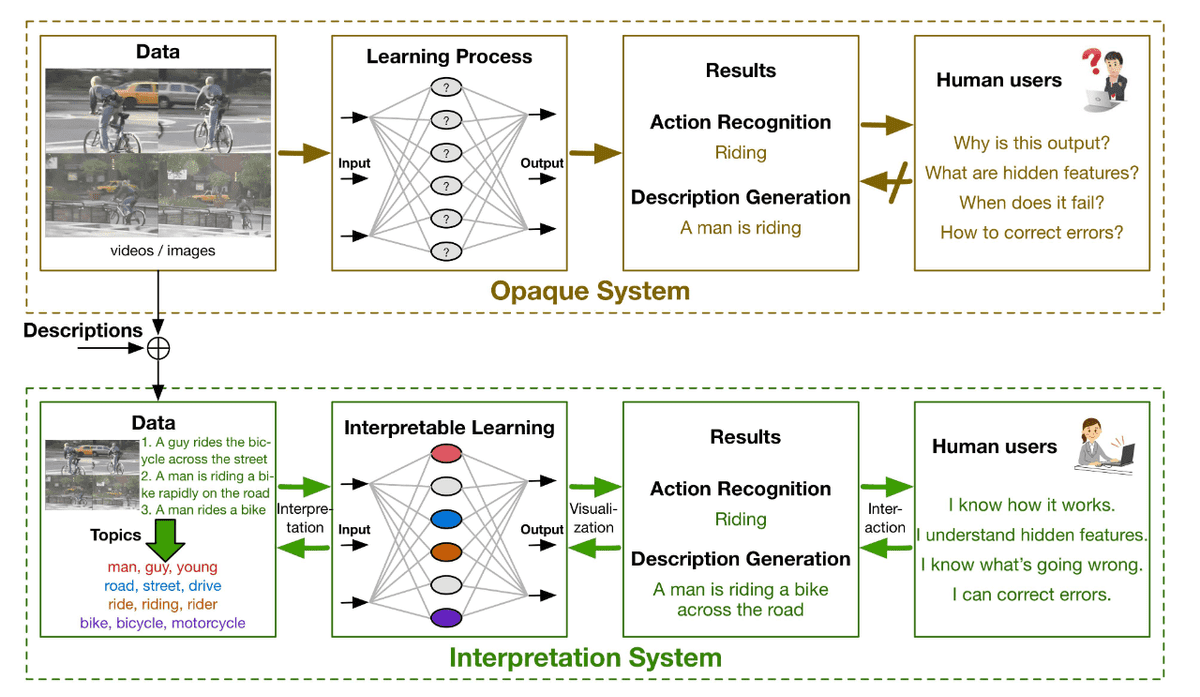
Interpetable training process of deep neural networks. Source: [7]

Visual dialog

In [6], the authors introduced a new task where an AI agent attempts a conversation with humans about visual content. A human makes questions about an image e.g., what color an object is, and the AI agent tries to answer. More specifically, the AI agent uses an encoder-decoder architecture that embeds the visual content and the history of the dialog to develop the next answer.

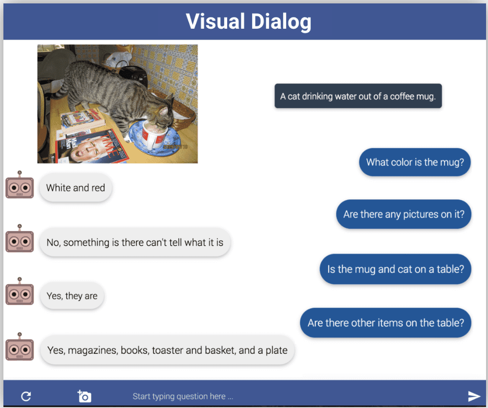
Example of visual dialog with an AI agent. Source: [7]

Numerical explanations

Concept Activation Vectors (CAVs)

Concept Activation Vectors (CAVs) [10] aim to explain the high-dimensional internal representations of neural networks. Given user-defined sets $\mathbf{P}_C$

S_{C,k,l} = \mathbf{h}_{k,l}(\nabla(f_{l}(\mathbf{x}))u_{C}^{l})

where $\mathbf{h}_{k,l}(\mathbf{x})$

Linear classifiers for features inspection

In [1], the authors proposed to train linear classifiers and inspect the features of any layer. A linear classifier is fitted to the intermediate layers to monitor the features and measures how suitable they are for classification.

Given the features $\mathbf{h}_{k}$

\mathbf{f}_{k}(\mathbf{h}_{k}) = softmax(\mathbf{Wh}_{k}+\mathbf{b})

The probe learns if the information from layer $k$ is useful for the classification of the input.

In general, it is proved that the most useful information is carried by the deeper layers of the network.

Local Interpretable Model-Agnostic Explanations (LIME)

Local Interpretable Model-Agnostic Explanations (LIME) [21] is able to interpret the predictions of any model-classifier $f$ by learning a local explainable model $g\in G$

\xi(g) = argmin L(f,g)+\Omega (g)

Applications

In this section, we will present explainable artificial intelligence methods that have been applied in some real-world tasks, such as autonomous driving and healthcare. These methods develop explainable algorithms to interpret results and improve their decisions or actions according to the task. Recent self-driving systems have adopted interpretation techniques to improve the actions of the autonomous driving system and reduce the risk of a crash. This is also important to increase the trust between humans and AI machines.

Explainable decisions for autonomous cars

In [26], the authors proposed a new explainable self-driving system inspired by the reactions and decisions of humans during driving. The proposed method consists of a CNN to extract features from the input image, while a global module generates the scene context from those features and provides information about the location of the objects. A local branch is employed to select the most important objects of the scene and associate them with the scene context to generate the actions and explanations. Finally, visual explanations are produced for the input image.

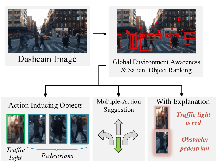
Example of actions and explanations of a self-driving system. Source: [26]

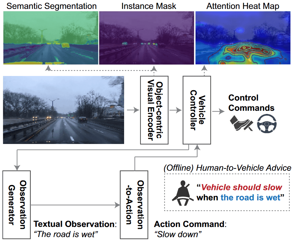
Similarly in [9], the authors proposed an autonomous driving architecture that is assisted and trained with the help of humans.

The system adopts a visual encoder to segment the objects of the input video stream. A vehicle controller is trained to generate spoken text of the commands, i.e., stops the car because the traffic light is red. In addition, the controller generates attention maps to highlight the important regions and explain their decisions. To further enhance the robustness of the system, an observation generator is employed that summarizes frames of the video and produces general observations that must be considered during driving. These observations are also fed to the vehicle controller to improve its decisions.

System overview. Source: [26]

Explainable medical systems

Artificial intelligence systems have also been implemented for medical applications. Deep learning has shown significant results especially in medical imaging and drug discovery. Recently, researchers have focused towards explainable medical systems to assist medical experts and provide useful explanations so that any expert can understand the predictions of a system. In [5], the authors focused on the detection of coronavirus from x-ray images. They proposed a deep convolutional network to extract features from images and detect if the patient is healthy or diagnosed with pneumonia or coronavirus. Then they use Grad-CAM [26] to provide visual explanations and mark the areas of the x-ray that are affected.

XAI frameworks

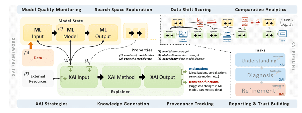
ExplAIner pipeline. Source: [24]

In this section, we will highlight some explainable AI frameworks that anyone can start using to interpet a machine learning model.

INNvestigate Neural networks

INNvestigate Neural networks [2] is a python package that has implemented a large variety of visual explanation methods such as LRP, CAM and PatternNet. The library contains examples with explanations of state-of-the-art models and is easy to use. The core and base functions of this framework allow rapid implementation of other methods.

explAIner

explAIner [24] is a unified framework that helps users to understand machine and deep learning models. In addition, the framework contains tools to analyze models using different explainable techniques. Then, these explanations are used in order to monitor and guide the optimization process and build better architectures. The explAIner is able to provide interactive graph visualization of a model, performance metrics and integrate high-level explainable methods to interpret it.

InterpetML

InterpetML [16] is an open-source Python library with many interpretability algorithms, which can be very easily integrated into the code. Then, we can easily understand the behavior of any model and compare different interpretation techniques.

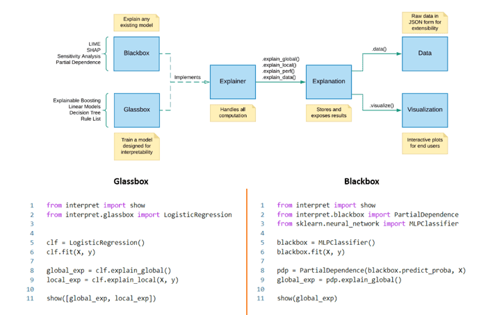
Usage of InterpetML framework. Source: [16]

Conclusion

In this article, we presented the major interpretation techniques and categorized them according to the explanation form. Some methods focus on providing visual explanations in the form of images or plots, while others provide textual or numerical explanations. Then, we described some of the latest explainable applications that are developed in demanding tasks like medical diagnosis and autonomous driving. Finally, we provided some well-known XAI frameworks that can be easily used by researchers for their algorithms.

Cited as:

@article{papastratis2021xai,
    title   = "Introduction to Explainable Artificial Intelligence (XAI)",
    author  = "Papastratis, Ilias",
    journal = "https://theaisummer.com/",
    year    = "2021",
    url     = "https://theaisummer.com/xai/"
  }

References

[1] Guillaume Alain and Yoshua Bengio.Understanding intermediate layers using linear classifier probes.arXiv preprintarXiv:1610.01644, 2016.

[2] Maximilian Alber, Sebastian Lapuschkin, Philipp Seegerer, MiriamHägele, Kristof T Schütt, Grégoire Montavon, Wojciech Samek,Klaus-Robert Müller, Sven Dähne, and Pieter-Jan Kindermans. iNNvestigate neural networks! J. Mach. Learn. Res., 20(93):1–8, 2019.

[3] Mathieu Aubry and Bryan C Russell. Understanding deep features with computer-generated imagery. InProceedings of the IEEE International Conference on Computer Vision, pages 2875–2883, 2015.

[4] Shane Barratt. Interpnet: Neural introspection for interpretable deeplearning.arXiv preprint arXiv:1710.09511, 2017.

[5] Luca Brunese, Francesco Mercaldo, Alfonso Reginelli, and Antonella Santone. Explainable deep learning for pulmonary disease and coronavirus covid-19 detection from x-rays. Computer Methods and Programs in Biomedicine, 196:105608, 2020.

[6] A Das, S Kottur, K Gupta, A Singh, D Yadav, S Lee, J Moura,D Parikh, and D Batra. Visual dialog. IEEE transactions on pat-tern analysis and machine intelligence, 2018.

[7] Yinpeng Dong, Hang Su, Jun Zhu, and Bo Zhang. Improving interpretability of deep neural networks with semantic information. InProceedings of the IEEE Conference on Computer Vision and Pattern Recognition, pages 4306–4314, 2017.27

[8] Andrej Karpathy, Justin Johnson, and Li Fei-Fei. Visualizing and understanding recurrent networks. 2016.

[9] Jinkyu Kim, Suhong Moon, Anna Rohrbach, Trevor Darrell, andJohn Canny. Advisable learning for self-driving vehicles by internal-izing observation-to-action rules. InProceedings of the IEEE/CVFConference on Computer Vision and Pattern Recognition, pages 9661–9670, 2020.

[10] Been Kim, Martin Wattenberg, Justin Gilmer, Carrie Cai, JamesWexler, Fernanda Viegas, et al. Interpretability beyond feature at-tribution: Quantitative testing with concept activation vectors (tcav).InInternational conference on machine learning, pages 2668–2677.PMLR, 2018.

[11] Devinder Kumar, Alexander Wong, and Graham W Taylor. Explaining the unexplained: A class-enhanced attentive response (clear) ap-proach to understanding deep neural networks. InProceedings of the IEEE Conference on Computer Vision and Pattern RecognitionWorkshops, pages 36–44, 2017.

[12] Ge Liu and David Gifford. Visualizing feature maps in deep neural networks using deepresolve a genomics case study. InICML Visual-ization Workshop, 2017.

[13] Liangzhi Li, Bowen Wang, Manisha Verma, Yuta Nakashima, Ryo Kawasaki, and Hajime Nagahara. Scouter: Slot attention-based classifier for explainable image recognition. arXiv preprintarXiv:2009.06138, 2020.

[14] Jiasen Lu, Jianwei Yang, Dhruv Batra, and Devi Parikh. Hierarchical question-image co-attention for visual question answering. Advances in neural information processing systems, 29:289–297, 2016.

[15] Laurens van der Maaten and Geoffrey Hinton. Visualizing data using t-sne. Journal of machine learning research, 9(Nov):2579–2605,2008.

[16] Harsha Nori, Samuel Jenkins, Paul Koch, and Rich Caruana. Interpretml: A unified framework for machine learning interpretability.arXiv preprint arXiv:1909.09223, 2019.

[19] José Antonio Oramas Mogrovejo, Kaili Wang, and Tinne Tuyte-laars. Visual explanation by interpretation: Improving visual feedback capabilities of deep neural networks. In https://iclr.cc/Conferences/2019/AcceptedPapersInitial. openReview, 2019.

[20] Paulo E Rauber, Samuel G Fadel, Alexandre X Falcao, and Alexan-dru C Telea. Visualizing the hidden activity of artificial neural networks. IEEE Transactions on Visualization and Computer Graphics,23(1):101–110, 2017.

[21] Marco Tulio Ribeiro, Sameer Singh, and Carlos Guestrin. ” Why should i trust you?” explaining the predictions of any classifier. InProceedings of the 22nd ACM SIGKDD international conference on knowledge discovery and data mining, pages 1135–1144, 2016.

[22] Ramprasaath R Selvaraju, Michael Cogswell, Abhishek Das, Ra-makrishna Vedantam, Devi Parikh, and Dhruv Batra. Grad-cam:Visual explanations from deep networks via gradient-based localization. InProceedings of the IEEE international conference on com-puter vision, pages 618–626, 2017.

[23] Wojciech Samek, Grégoire Montavon, Alexander Binder, Sebastian Lapuschkin, and Klaus-Robert Müller. Interpreting the predictions of complex ml models by layer-wise relevance propagation. arXivpreprint arXiv:1611.08191, 2016.

[24] Thilo Spinner, Udo Schlegel, Hanna Schäfer, and Mennatallah El-Assady. explainer: A visual analytics framework for interactive and explainable machine learning. IEEE transactions on visualization and computer graphics, 26(1):1064–1074, 2019.

[25] Jayaraman J Thiagarajan, Bhavya Kailkhura, Prasanna Sattigeri,and Karthikeyan Natesan Ramamurthy. Treeview: Peeking into deep neural networks via feature-space partitioning. arXiv preprintarXiv:1611.07429, 2016.

[26] Yiran Xu, Xiaoyin Yang, Lihang Gong, Hsuan-Chu Lin, Tz-YingWu, Yunsheng Li, and Nuno Vasconcelos. Explainable object-induced action decision for autonomous vehicles. InProceedings of 30BIBLIOGRAPHY the IEEE/CVF Conference on Computer Vision and Pattern Recog-nition, pages 9523–9532, 2020.

[27] Matthew D Zeiler and Rob Fergus. Visualizing and understanding convolutional networks. In European conference on computer vi-sion, pages 818–833. Springer, 2014.

[28] Bolei Zhou, Aditya Khosla, Agata Lapedriza, Aude Oliva, and Anto-nio Torralba. Learning deep features for discriminative localization. In Proceedings of the IEEE conference on computer vision and pat-tern recognition, pages 2921–2929, 2016.

[29] Yanzhao Zhou, Yi Zhu, Qixiang Ye, Qiang Qiu, and Jianbin Jiao. Weakly supervised instance segmentation using class peak response. InProceedings of the IEEE Conference on Computer Vision and Pat-tern Recognition, pages 3791–3800, 2018.

* Disclosure: Please note that some of the links above might be affiliate links, and at no additional cost to you, we will earn a commission if you decide to make a purchase after clicking through.

Source link