
In the Part 1 of Introduction to Neural Networks we learned about one of the simplest artificial neuron called McCulloch-Pitts neuron and implemented it in python.
The problem with M-P neuron is that there is actually no learning involved. The weights are set manually.
In this article we’ll see Perceptron which is an improvement from the M-P neuron. Unlike M-P neuron the perceptron can learn the weights over time.
We will also see how to train a Perceptron from scratch to classify logical operations like AND or OR.
Perceptron:
A perceptron is basically a binary classifier. It is an algorithm for determining a hyperplane that separates two categories of data.
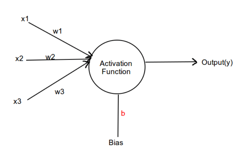
A typical perceptron will have
-
- Inputs
- Weights and Bias
- Activation function

The perceptron receives input data multiplied by random weights and adds bias to it. A bias functions like an input node that always produce constant value.
\text { Weighted sum }=\quad \sum_{i=1}^{m} \mathrm{x}_{\mathrm{i}} \mathrm{W}_{\mathrm{i}}+\mathrm{b}
\text { Weighted sum }=x_{1} w_{1}+x_{2} w_{2}+x_{3} w_{3}+b
Then an activation function will be applied to the weighted sum. The weighted sum is nothing but the sum of all the inputs multiplied by its weights + bias.
Here we are going to use unit step or heaviside activation function. It is a threshold based activation function.

f(x)=\left\{\begin{array}{ll}<br />
0 & \text { for } x<0 \\<br />
1 & \text { for } x \geq 0<br />
\end{array}\right.
If the input value is greater than 0 then it returns 1, else it returns 0.
Perceptron Learning:
Now let’s see the exact steps involved in training a perceptron.
Training a perceptron is simple and straightforward. We need to obtain a set of weights that classifies each instance in our training set.
The first step is to initialize the weights and bias randomly.
Then we have to calculate the net input by multiplying the input with the weights along with the bias.
y_{i n}=\sum_{i=1}^{m} x_{i} w_{i}+b
Then we have to apply activation function over the net input. Here we use step function which squashes the input between 0 and 1.
y = Φ(yin)
And in the final step if the predicted value is not equal to the targeted value then we have to update the weights and bias.
error = t – y
Here t is the target value and y is the predicted value.
The weights and bias update are as follows:
wi(new) = wi(old) + alpha * error * xi
b(new) = b(old) + alpha * error
The alpha here is the learning rate.
Implementation:
Now let’s train a Perceptron to predict the output of a logical OR gate.
|
1 2 3 4 5 6 7 8 9 10 11 12 13 14 15 16 17 18 19 20 21 22 23 24 25 26 27 28 29 30 31 32 33 34 35 36 37 38 39 40 41
|
import numpy as np
#Activation Function def step(x): return 1 if x > 0 else 0
#Training Data data = [[0,0], [0,1], [1,0], [1,1]]
#Target Values y = [0, 1, 1, 1]
#Initialising weights and bias w = np.random.randn(2) b = np.random.randn() epochs = 30 alpha = 0.1
#loop over desired number of epochs for i in range(epochs): #loop over individual data point for(x, target) in zip(data, y): #performing the dot product between the input data and the weights z = sum(x * w) + b #passing the net input through the activation function pred = step(z) #calculating the error error = target – pred #updating the weights and bias for index,value in enumerate(x): w[index] += alpha * error * value b += alpha * error
#Testing test = [0, 1] u = w[0] * test[0] + w[1] * test[1] + b pred = step(u) print(pred) |
Now let’s try it for AND operator. We just need to change the target values.
y = [0, 0, 0, 1]
Now if we run the program we will get the output as 0. Since 0 AND 1 is 0
You can try changing the test values as [0,0],[1,0] or [1,1].
Now if you try to classify XOR with the perceptron by changing the target values(y) no matter how many epochs you train the network you will never able to classify since it is not linearly classifiable.
Then how can we classify functions which are not linearly separable. For that, we need multi-layer perceptron which has more layers than a normal perceptron.
CONCLUSION:
In this article we have learned what a perceptron is and how to implement them from scratch in python.
A perceptron is a binary classifier which determines a hyperplane that separates two categories of data. However the problem with perceptron is that it is a linear classifier. It cannot deal with non-linear problems.
In the next part we’ll learn about multi-layered perceptron which can deal with non-linear problems.