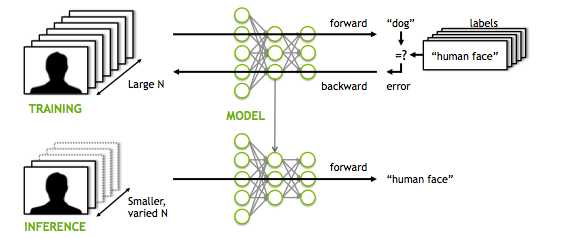
In this part we are going to examine how we can improve our neural network library by adding a convolutional neural network structure to use on a dataset of images.
No one can argue that convolutional neural networks are the best way to classify and train images and this is why they have so much use in computer vision systems. The goal, of course, is to use again GPU’s and OpenCL as ConvNets require more computing resourses and memory than plain fully connected networks.
Let’s begin.
First of all , we have to remember that CovNets in their simpler forms consist of a convolutional layer, a pooling layer and a fully connected layer. Luckily we have implemented the last one . So all it remains are the two first.
Convolutional layer
This time i am not gonna get into much details about the C++ part and how we will build the basic structure of our ConvNet (i did that in the first part for Fully Connected Layers) , but i will dive on the kernels code, which i think is the most interesting. In those layers, we convolve the input image with a small size kernel and we acquire the fearure map.
kernel void convolve(global float *image, global Filter* filters, global float * featMap,int filterWidth,int inWidth,int featmapdim){
const int xIn=get_global_id(0);
const int yIn=get_global_id(1);
const int z=get_global_id(2);
float sum=0;
for (int r=0;r<filterWidth;r++){
for (int c=0;c<filterWidth;c++){
sum+= filters[z].weights[c*filterWidth +r]*image[(xIn+c)+inWidth*(yIn+r)];
}
}
sum +=filters[z].bias;
featMap[(xIn+yIn*featmapdim +z*featmapdim*featmapdim)] =relu(sum);
}
As you can tell, we are based on the hypothesis that each pixel of the feature map is calculated parallelly as it is inherently independent from all the others. So if we have an image 28×28 and we use a kernel 5×5, we will need 24×24=576 threads to run simultaneously.
The backward propagation is a little more tricky because there are not many online resourses to actually provide the equations for a convolutional layer.
If we translate the above in c code we get:
kernel void deltas(global Node * nodes,global Node * nextnodes,global float *deltas,global int *indexes,int dim,int nextnumNodes,int pooldim){
const int xIn=get_global_id(0);
const int yIn=get_global_id(1);
const int z=get_global_id(2);
int i = xIn+yIn*pooldim +z*pooldim*pooldim;
float delta = 0;
for (int j = 0; j !=nextnumNodes; j++)
delta += nextnodes[j].delta * nextnodes[j].weights[i];
delta *= devsigmoid(nodes[i].output);
for(int r=0;r<2;r++){
for(int c=0;c<2;c++){
if((c*2+r)==indexes[i])
deltas[(2*xIn+r)+(2*yIn+c)*dim+z*dim*dim]=delta;
}
}
}
kernel void backpropcnn( global float* featMap,global float* deltas,global Filter* filters,int featmapdim,int imagedim,int filterdim,float a,global float* Image){
const int xIn=get_global_id(0);
const int yIn=get_global_id(1);
const int z=get_global_id(2);
float sum=0;
for (int r=0;r<featmapdim;r++){
for (int c=0;c<featmapdim;c++){
sum+= deltas[(c+r*featmapdim +z*featmapdim*featmapdim)]*Image[(xIn+r)+imagedim *(yIn+c)];
}
}
filters[z].weights[(xIn+filterdim *yIn)] -=a*sum;
}
Pooling layer
The pooling layers is just a down sampling of the feature map into a new map with smaller size. There are two kind of pooling : Average and max pooling with the second being the most used. In max pooling, we just define a filter (usually of size 2×2) and we apply it on the feture map. The goal of the filter is to simply extract the maximum value of the filter window in the image.
kernel void pooling( global float* prevfeatMap,global float* poolMap,global int* indexes,int Width,int pooldim){
const int xIn=get_global_id(0);
const int yIn=get_global_id(1);
const int z=get_global_id(2);
float max=0;
int index = 0;
for (int r=0;r<2;r++){
for (int c=0;c<2;c++){
if(prevfeatMap[(yIn+c)*Width*z +(xIn+r)]>max){
max=prevfeatMap[(yIn+c)*Width*z +(xIn+r)];
index=c*2+r;
}
}
}
poolMap[(xIn+yIn*pooldim +z*pooldim*pooldim)]=max;
indexes[(xIn+yIn*pooldim +z*pooldim*pooldim)]=index;
}
As fas as the backward propagation is concerned, there are no actual gradient calculations. All we need to do is to upsample the matrix. In fact we pass the gradient on the “winning unit” of the forward propagation. That is the reason why we build and indexes matrix in the above snippet before, in which we keep the position of all ” winning units”. This functionality is visible on the “deltas” function, which is responsible for the calculation of the gradient errors.
To run the kernels code, we follow the next steps:
-
Pass the data in matrix format (OpenCV can be used for that)
-
Define the cl: Buffers and the cl::Kernels
-
Run the kernels with the following code:
convKern.setArg(0, d_InputBuffer);convKern.setArg(1, d_FiltersBuffer);convKern.setArg(2, d_FeatMapBuffer);
convKern.setArg(3, filterdim);convKern.setArg(4, inputdim);convKern.setArg(5, featmapdim);
err = (OpenCL::clqueue).enqueueNDRangeKernel(convKern, cl::NullRange,
cl::NDRange(featmapdim, featmapdim, convLayer.numOfFilters),
cl::NullRange);
poolKern.setArg(0, d_FeatMapBuffer);poolKern.setArg(1, d_PoolBuffer);poolKern.setArg(2, d_PoolIndexBuffer);
poolKern.setArg(3, featmapdim);poolKern.setArg(4, pooldim);
err = (OpenCL::clqueue).enqueueNDRangeKernel(poolKern, cl::NullRange,
cl::NDRange(pooldim, pooldim, convLayer.numOfFilters),
cl::NullRange);
deltasKern.setArg(0, d_layersBuffers[0]);deltasKern.setArg(1, d_layersBuffers[1]);deltasKern.setArg(2, d_deltasBuffer);deltasKern.setArg(3, d_PoolIndexBuffer);
deltasKern.setArg(4, featmapdim);deltasKern.setArg(5, h_netVec[1]);deltasKern.setArg(6, pooldim);
err = (OpenCL::clqueue).enqueueNDRangeKernel(deltasKern, cl::NullRange,
cl::NDRange(pooldim, pooldim,convLayer.numOfFilters),
cl::NullRange);
backpropcnnKern.setArg(0, d_FeatMapBuffer);backpropcnnKern.setArg(1, d_rotatedImgBuffer);backpropcnnKern.setArg(2, d_FiltersBuffer);
backpropcnnKern.setArg(3, featmapdim);backpropcnnKern.setArg(4, inputdim);backpropcnnKern.setArg(5, filterdim);
backpropcnnKern.setArg(6, lr);backpropcnnKern.setArg(7, d_InputBuffer);
err = (OpenCL::clqueue).enqueueNDRangeKernel(backpropcnnKern, cl::NullRange,
cl::NDRange(filterdim, filterdim,convLayer.numOfFilters),
cl::NullRange);
It was not that bad right? If you have to get only one thing from the two posts is that neural networks and deep learning in general is nothing more than operations between matrixes that try to approximate a mathematical function. Even if that function is how to drive a car.
We saw that building a Neural network library from scratch and even program them to run on GPU’s is not something quite difficult. All you need is a basic understanding of linar algebra and a a glimpse of how graphical processing units work.
I should remind you one more that the complete code can be found on my repository on github. Neural netwok library
* Disclosure: Please note that some of the links above might be affiliate links, and at no additional cost to you, we will earn a commission if you decide to make a purchase after clicking through.


