Self-supervised learning aims to extract representation from unsupervised visual data and it’s super famous in computer vision nowadays. This article covers the SWAV method, a robust self-supervised learning paper from a mathematical perspective. To that end, we provide insights and intuitions for why this method works. Additionally, we will discuss the optimal transport problem with entropy constraint and its fast approximation that is a key point of the SWAV method that is hidden when you read the paper.
In any case, if you want to learn more about general aspects of self-supervised learning, like augmentation, intuitions, softmax with temperature, and contrastive learning, consult our previous article.
SWAV Method overview
Definitions
Let two image features and be two different augmentations of the same image. The image features are generated by taking stochastic augmentations of the same image .

Source: BYOL
-
Our actual targets: Let and be the respective codes of the image views. Codes can be regarded as a soft class of the image.
-
Prototypes: consider a set of prototypes lying in the unit sphere. The prototypes are trainable vectors that will move based on the dataset’s over-represented (frequent) features. If the dataset consists only of cars, then it will be the most part of a car like a wheel, car windows, car lights, mirrors etc. One way to think about it is as a low-dimensional projection of the whole dataset.

Source: SWAV paper, Caron et al 2020
Clusters and prototypes are used interchangeably throughout this article. Don’t confuse it with “codes” though! Nonetheless, codes and assignments are also used interchangeably.
SWAV compares the features and using the intermediate codes (soft classes) and . For now, ignore how we compute the codes. Keep it as a target in a standard supervised classification problem.
Intuition: If and capture similar information, we can predict the code (soft class) from the other feature . In other words, if the two views share the same semantics, their targets (codes) will be similar. This is the whole “swapping” idea.
Source: SWAV’s github page
Difference between SWAV and SimCLR
In contrastive learning methods, the features from different transformations of the same images are compared directly to each other. SWAV does not directly compare image features. Why?
In SwAV, there is the intermediate “codes” step (). To create the codes (targets), we need to assign the image features to prototype vectors. We then solve a “swapped” prediction problem wherein the codes (targets) are altered for the two image views.

Source: SWAV paper, Caron et al 2020
Prototype vectors are learned but they are still in the unit sphere area, meaning their L2 norm will be 1.
The unit sphere and its implications
By definition, a unit sphere is the set of points with L2 distance equal to 1 from a fixed central point, here the origin. Note that this is different from a unit ball, where the L2 distance is less than or equal to 1 from the centre.
Moving on the surface of the sphere corresponds to a smooth change in assignments. In fact many self-supervised methods are using this L2-norm trick, and especially contrastive methods. SWAV also applies L2-normalization to the features as well as to the prototypes throughout training.
SWAV method Steps
Let’s recap the steps of SWAV:
-
Create views from input image using a set of stochastic transformations
-
Calculate image feature representations
-
Calculate softmax-normalized similarities between all and :
-
Calculate code matrix iteratively. We intentionally ignored this part. See further on for this step.
-
Calculate cross-entropy loss between representation , aka and the code of representation , aka
-
Average loss between all views.

Source: SWAV paper, Caron et al 2020
Again, notice the difference between cluster assignments (codes) and cluster prototype vectors (). Here is a detailed explanation of the loss function:
Digging into SWAV’s math: approximating Q
Understanding the Optimal Transport Problem with Entropic Constraint
As discussed, the code vectors act as a target in the cross-entropy loss term. In SWAV, these code vectors are computed online during every iteration. Online means that we approximate in each forward pass by an iterative process. No gradients and backprop to estimate .
For prototypes and batch size , the optimal code matrix is defined as the solution to an optimal transport problem with entropic constraint. The solution is approximated using the iterative Sinkhorn-Knopp algorithm .
For a formal and very detailed formulation, analysis and solution of said problem, I recommend having a look at the paper .
For SwAV, we define the optimal code matrix as:
with being the entropy and being a hyperparameter of the method.
The trace is defined to be the sum of the elements on the main diagonal.
A matrix from the set is constrained in three ways:
-
All its entries have to be positive.
-
The sum of each row has to be
-
The sum of each column has to be .
-
Note that this also implies that the sum of all entries to be , hence these matrices allow for a probabilistic interpretation, for example, w.r.t. Entropy. However, it’s not a stochastic matrix.
A simple matrix in this set is a matrix whose entries are all , which corresponds to a uniform distribution over all entries. This matrix maximizes the entropy .
With a good intuition on the set , we can examine the target function.
Optimal transport without entropy
Ignoring the entropy-term for now, we can go step-by-step through the first term
Since both and are L2 normalized, the matrix product computes the cosine similarity scores between all possible combinations of feature vectors and prototypes .
The first column of contains the similarity scores for the first feature vector and all prototypes.
This means that the first diagonal entry of is a weighted sum of the similarity scores of . For 2 prototypes and batch size 3 the first diagonal element will be:
While its entropy term will be:
Similarly, the second diagonal entry of is a weighted sum of the similarity scores for with different weights.
Doing this for all diagonal entries and taking the sum results in .
Intuition: While the optimal matrix is highly non-trivial, it is easy to see that will assign large weights to larger similarity scores and small weights to smaller ones while conforming to the row-sum and column-sum constraint.
Based on this design, such a method would be more biased to mode collapse by choosing one prototype than collapsing to a uniform distribution.
Solution? Enforcing entropy to the rescue!
The entropy constraint
So why do we need the entropy term at all?
Well, while the resulting code vectors are already a ‘soft’ target compared to one-hot vectors (in SimCLR), the addition of the entropy term in the target function gives us control over the smoothness of the solution.
For the solution tends towards the trivial solution where all entries of are . Basically, all feature vectors are assigned uniformly to all prototypes.
When we have no smoothness term to further regularize .
Finally, small values for result in a slightly smoothed .
Revisiting the constraints for , the row-sum and column-sum constraints imply an equal amount of total weight is assigned to each prototype and each feature vector respectively.
The constraints impose a strong regularization that results in avoiding mode collapse, where all feature vectors are assigned to the same prototype all the time.
Online estimation of Q* for SWAV
What is left now is to compute in every iteration of the training process, which luckily turns out to be very efficient using the results of .
Using Lemma 2 from page 5, we know that the solution takes the form:
where and act as column and row normalization vectors respectively. An exact computation here is inefficient. However, the algorithm provides a fast, iterative alternative. We can initialize a matrix as the exponential term from and then alternate between normalizing the rows and columns of this matrix.
Sinkhorn-Knopp Code analysis
Here is the pseudocode, given by the authors on the approximation of Q from the similarity scores:
def sinkhorn(scores, eps=0.05, niters=3):
Q = exp(scores / eps).T
Q /= sum(Q)
K, B = Q.shape
u, r, c = zeros(K), ones(K) / K, ones(B) / B
for _ in range(niters):
u = sum(Q, dim=1)
Q *= (r / u).unsqueeze(1)
Q *= (c / sum(Q, dim=0)).unsqueeze(0)
return (Q / sum(Q, dim=0, keepdim=True)).T
To approximate , we take as input only the similarity score matrix and output our estimation for .
Intuition on the clusters/prototypes
So what is actually learned in these clusters/prototypes?
Well, the prototypes’ main purpose is to summarize the dataset. So SWAV is still a form of contrastive learning. In fact, it can also be interpreted as a way of contrasting image views by comparing their cluster assignments instead of their features.
Ultimately, we contrast with the clusters and not the whole dataset. SimCLR uses batch information, called negative samples, but it is not always representative of the whole dataset. That makes the SWAV objective more tractable.
This can be observed from the experiments. Compared to SimCLR, SWAV pretraining converges faster and is less sensitive to the batch size. Moreover, SWAV is not that sensitive to the number of clusters. Typically 3K clusters are used for ImageNet. In general, it is recommended to use approximately one order of magnitude larger than the real class labels. For STL10 which has 10 classes, 512 clusters would be enough.
The multi-crop idea: augmenting views with smaller images
Every time I read about contrastive self-supervised learning methods I think, why just 2 views? Well, the obvious question is answered in the SWAV paper also.

Multi-crop. Source: SWAV paper, Caron et al 2020
To this end, SwAV proposes a multi-crop augmentation strategy where the same image is cropped randomly with 2 global (i.e. 224×224) views and local (i.e. 96×96) views.
As shown below, multi-crop is a very general trick to improve self-supervised learning representations. It can be used out of the box for any method with surprisingly good results ~2% improvement on SimCLR!

Source: SWAV paper, Caron et al 2020
The authors also observed that mapping small parts of a scene to more global views significantly boosts the performance.
Results
To evaluate the learned representation of , the backbone model i.e. Resnet50 is frozen. A single linear layer is trained on top. This is a fair comparison for the learned representations, called linear evaluation. Below are the results of SWAV compared to other state-if-the-art-methods.

(left) Comparison between clustering-based and contrastive instance methods and
impact of multi-crop. (right) Performance as a function of epochs. Source: SWAV paper, Caron et al 2020
Left: Classification accuracy on ImageNet is reported. The linear layers are trained on frozen features from different self-supervised methods with a standard ResNet-50. Right: Performance of wide ResNets-50 by factors of 2, 4, and 5.
Conclusion
In this post an overview of SWAV and its hidden math is provided. We covered the details of optimal transport with and without the entropy constraint. This post would not be possible without the detailed mathematical analysis of Tim.
Finally you can check out this interview on SWAV by its first author (Mathilde Caron).
For further reading, take a look at self-supervised representation learning on videos or SWAV’s experimental report. You can even run your own experiments with the official code if you have a multi-GPU machine!
Finally, I have to say that I’m a bit biased on the work of FAIR on visual self-supervised learning. This team really rocks!
References
-
SWAV Paper
-
SWAV Code
-
Ref paper on optimal transport
-
SWAV’s Report in WANDB
Cite as:
@article{kaiser2021swav,
title = "Understanding SWAV: self-supervised learning with contrasting cluster assignments",
author = "Kaiser, Tim and Adaloglou, Nikolaos",
journal = "https://theaisummer.com/",
year = "2021",
howpublished = {https://theaisummer.com/swav/},
}

* Disclosure: Please note that some of the links above might be affiliate links, and at no additional cost to you, we will earn a commission if you decide to make a purchase after clicking through.