I was very curious to see how JAX is compared to Pytorch or Tensorflow. I figured that the best way for someone to compare frameworks is to build the same thing from scratch in both of them. And that’s exactly what I did. In this article, I am developing a Variational Autoencoder with JAX, Tensorflow and Pytorch at the same time. I will present the code for each component side by side in order to find differences, similarities, weaknesses and strengths.
Shall we begin?
Prologue
Some things to note before we explore the code:
-
I will use Flax on top of JAX, which is a neural network library developed by Google. It contains many ready-to-use deep learning modules, layers, functions, and operations
-
For the Tensorflow implementation, I will rely on Keras abstractions.
-
For Pytorch, I will use the standard
nn.module.
Because most of us are somewhat familiar with Tensorflow and Pytorch, we will pay more attention in JAX and Flax. That’s why I will explain things along the way that may be unfamiliar to many. So you can consider this article as a light tutorial on Flax as well.
Also, I assume that you are familiar with the basic principles behind VAEs. If not, you can advise my previous article on latent variable models. If everything seems clear, let’s continue.
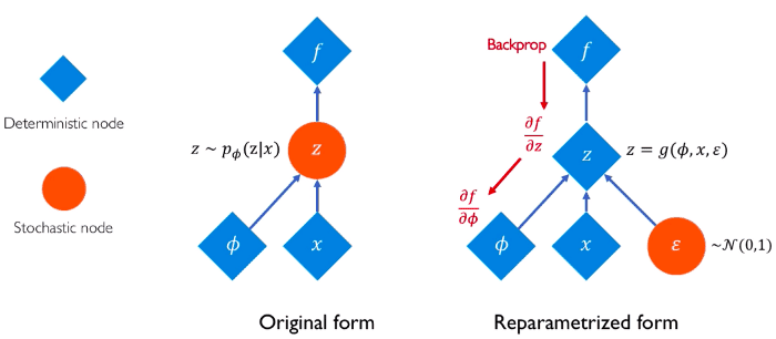
Quick recap: The vanilla Autoencoder consists of an Encoder and a Decoder. The encoder converts the input to a latent representation and the decoder tries to reconstruct the input based on that representation. In Variational Autoencoders, stochasticity is also added to the mix in terms that the latent representation provides a probability distribution. This is happening with the reparametrization trick.
The encoder
For the encoder, a simple linear layer followed by a RELU activation should be enough for a toy example. The output of the layer will be both the mean and standard deviation of the probability distribution.
The basic building block of the Flax API is the Module abstraction, which is what we’ll use to implement our encoder in JAX. The module is part of the linen subpackage. Similar to Pytorch’s nn.module, we again need to define our class arguments. In Pytorch, we are used to declaring them inside the __init__ function and implementing the forward pass inside the forward method. In Flax, things are a little different. Arguments are defined either as dataclass attributes or as method arguments. Usually, fixed properties are defined as dataclass arguments while dynamic properties as method arguments. Also instead of implementing a forward method, we implement __call__
The Dataclass module is introduced in Python 3.7 as a utility tool to make structured classes especially for storing data. These classes hold certain properties and functions to deal specifically with the data and its representation. They also reduce a lot of boilerplate code compared to regular classes.
So to create a new module in Flax, we need to:
-
Initialize a class that inherits
flax.linen.nn.Module -
Define the static arguments as dataclass arguments
-
Implement the forward pass inside the
__call_method.
To tie the arguments with the model and being able to define submodules directly within the module, we also need to annotate the __call__ method with @nn.compact.
Note that instead of using dataclass arguments and the @nn.compact annotation, we could have declared all arguments inside a setup method in the exact same way as we do in Pytorch’s or Tensorflow’s __init__.
import numpy as np
import jax
import jax.numpy as jnp
from jax import random
from flax import linen as nn
from flax import optim
class Encoder(nn.Module):
latents: int
@nn.compact
def __call__(self, x):
x = nn.Dense(500, name='fc1')(x)
x = nn.relu(x)
mean_x = nn.Dense(self.latents, name='fc2_mean')(x)
logvar_x = nn.Dense(self.latents, name='fc2_logvar')(x)
return mean_x, logvar_x
import tensorflow as tf
from tensorflow.keras import layers
class Encoder(layers.Layer):
def __init__(self,
latent_dim =20,
name='encoder',
**kwargs):
super(Encoder, self).__init__(name=name, **kwargs)
self.enc1 = layers.Dense(500, activation='relu')
self.mean_x = layers.Dense(latent_dim)
self.logvar_x = layers.Dense(latent_dim)
def call(self, inputs):
x = self.enc1(inputs)
z_mean = self.mean_x(x)
z_log_var = self.logvar_x(x)
return z_mean, z_log_var
import torch
import torch.nn.functional as F
class Encoder(torch.nn.Module):
def __init__(self, latent_dim=20):
super(Encoder, self).__init__()
self.enc1 = torch.nn.Linear(784, 500)
self.mean_x = torch.nn.Linear(500,latent_dim)
self.logvar_x = torch.nn.Linear(500, latent_dim)
def forward(self,inputs):
x = self.enc1(inputs)
x= F.relu(x)
z_mean = self.mean_x(x)
z_log_var = self.logvar_x(x)
return z_mean, z_log_var
A few more things to notice here before we proceed:
-
Flax’s
nn.linenpackage contains most deep learning layers and operation such asDense,relu, and many more -
The code in Flax, Tensorflow, and Pytorch is almost indistinguishable from each other.
The decoder
In a very similar fashion, we can develop the decoder in all 3 frameworks. The decoder will be two linear layers that receive the latent representation and output the reconstructed input.
Again the implementations are very similar.
class Decoder(nn.Module):
@nn.compact
def __call__(self, z):
z = nn.Dense(500, name='fc1')(z)
z = nn.relu(z)
z = nn.Dense(784, name='fc2')(z)
return z
class Decoder(layers.Layer):
def __init__(self,
name='decoder',
**kwargs):
super(Decoder, self).__init__(name=name, **kwargs)
self.dec1 = layers.Dense(500, activation='relu')
self.out = layers.Dense(784)
def call(self, z):
z = self.dec1(z)
return self.out(z)
class Decoder(torch.nn.Module):
def __init__(self, latent_dim=20):
super(Decoder, self).__init__()
self.dec1 = torch.nn.Linear(latent_dim, 500)
self.out = torch.nn.Linear(500, 784)
def forward(self,z):
z = self.dec1(z)
z = F.relu(z)
return self.out(z)
Variational Autoencoder
To combine the encoder and the decoder, let’s have one more class, called VAE, that will represent the entire architecture. Here we also need to write some code for the reparameterization trick. Overall we have: the latent variable from the encoder is reparameterized and fed to the decoder, which produces the reconstructed input.
As a reminder, here is an intuitive image that explains the reparameterization trick:

Source: Alexander Amini and Ava Soleimany, Deep Generative Modeling | MIT 6.S191, http://introtodeeplearning.com/
Notice that this time, in JAX we make use of the setup method instead of the nn.compact annotation. Also, check out how similar the reparameterization functions are. Sure each framework uses its own functions and operations but the general image is almost identical.
class VAE(nn.Module):
latents: int = 20
def setup(self):
self.encoder = Encoder(self.latents)
self.decoder = Decoder()
def __call__(self, x, z_rng):
mean, logvar = self.encoder(x)
z = reparameterize(z_rng, mean, logvar)
recon_x = self.decoder(z)
return recon_x, mean, logvar
def reparameterize(rng, mean, logvar):
std = jnp.exp(0.5 * logvar)
eps = random.normal(rng, logvar.shape)
return mean + eps * std
def model():
return VAE(latents=LATENTS)
class VAE(tf.keras.Model):
def __init__(self,
latent_dim=20,
name='vae',
**kwargs):
super(VAE, self).__init__(name=name, **kwargs)
self.encoder = Encoder(latent_dim=latent_dim)
self.decoder = Decoder()
def call(self, inputs):
z_mean, z_log_var = self.encoder(inputs)
z = self.reparameterize(z_mean, z_log_var)
reconstructed = self.decoder(z)
return reconstructed, z_mean, z_log_var
def reparameterize(self, mean, logvar):
eps = tf.random.normal(shape=mean.shape)
return mean + eps * tf.exp(logvar * .5)
class VAE(torch.nn.Module):
def __init__(self, latent_dim=20):
super(VAE, self).__init__()
self.encoder = Encoder(latent_dim)
self.decoder = Decoder(latent_dim)
def forward(self,inputs):
z_mean, z_log_var = self.encoder(inputs)
z = self.reparameterize(z_mean, z_log_var)
reconstructed = self.decoder(z)
return reconstructed, z_mean, z_log_var
def reparameterize(self, mu, log_var):
std = torch.exp(0.5 * log_var)
eps = torch.randn_like(std)
return mu + (eps * std)
Loss and Training step
Things are starting to differ when we begin implementing the training step and the loss function. But not by much.
-
In order to fully take advantage of JAX capabilities, we need to add automatic vectorization and XLA compiling to our code. This can be done easily with the help of
vmapandjitannotations. -
Moreover, we have to enable automatic differentiation, which can be accomplished with the
grad_fntransformation -
We use the
flax.optimpackage for optimization algorithms
Another small difference that we need to be aware of is how we pass data to our model. This can be achieved through the apply method in the form of model().apply({'params': params}, batch, z_rng), where batch is our training data.
@jax.vmap
def kl_divergence(mean, logvar):
return -0.5 * jnp.sum(1 + logvar - jnp.square(mean) - jnp.exp(logvar))
@jax.vmap
def binary_cross_entropy_with_logits(logits, labels):
logits = nn.log_sigmoid(logits)
return -jnp.sum(labels * logits + (1. - labels) * jnp.log(-jnp.expm1(logits)))
@jax.jit
def train_step(optimizer, batch, z_rng):
def loss_fn(params):
recon_x, mean, logvar = model().apply({'params': params}, batch, z_rng)
bce_loss = binary_cross_entropy_with_logits(recon_x, batch).mean()
kld_loss = kl_divergence(mean, logvar).mean()
loss = bce_loss + kld_loss
return loss, recon_x
grad_fn = jax.value_and_grad(loss_fn, has_aux=True)
_, grad = grad_fn(optimizer.target)
optimizer = optimizer.apply_gradient(grad)
return optimizer
def kl_divergence(mean, logvar):
return -0.5 * tf.reduce_sum(
1 + logvar - tf.square(mean) -
tf.exp(logvar), axis=1)
def binary_cross_entropy_with_logits(logits, labels):
logits = tf.math.log(logits)
return - tf.reduce_sum(
labels * logits +
(1-labels) * tf.math.log(- tf.math.expm1(logits)),
axis=1
)
@tf.function
def train_step(model, x, optimizer):
with tf.GradientTape() as tape:
recon_x, mean, logvar = model(x)
bce_loss = tf.reduce_mean(binary_cross_entropy_with_logits(recon_x, batch))
kld_loss = tf.reduce_mean(kl_divergence(mean, logvar))
loss = bce_loss + kld_loss
print(loss, kld_loss, bce_loss)
gradients = tape.gradient(loss, model.trainable_variables)
optimizer.apply_gradients(zip(gradients, model.trainable_variables))
def final_loss(reconstruction, train_x, mu, logvar):
BCE = torch.nn.BCEWithLogitsLoss(reduction='sum')(reconstruction, train_x)
KLD = -0.5 * torch.sum(1 + logvar - mu.pow(2) - logvar.exp())
return BCE + KLD
def train_step(train_x):
train_x = torch.from_numpy(train_x)
optimizer.zero_grad()
reconstruction, mu, logvar = model(train_x)
loss = final_loss(reconstruction, train_x, mu, logvar)
running_loss += loss.item()
loss.backward()
optimizer.step()
Remember that VAEs are trained by maximizing the evidence lower bound, known as ELBO.
Training loop
Finally, it’s time for the entire training loop which will execute the train_step function iteratively.
In Flax, the model has to be initialized before training, which is done by the init function such as: params = model().init(key, init_data, rng)['params']. A similar initialization is necessary for the optimizer as well: optimizer = optim.Adam( learning_rate = LEARNING_RATE ).create( params ).
jax.device_put is used to transfer the optimizer into the GPU’s memory.
rng = random.PRNGKey(0)
rng, key = random.split(rng)
init_data = jnp.ones((BATCH_SIZE, 784), jnp.float32)
params = model().init(key, init_data, rng)['params']
optimizer = optim.Adam(learning_rate=LEARNING_RATE).create(params)
optimizer = jax.device_put(optimizer)
rng, z_key, eval_rng = random.split(rng, 3)
z = random.normal(z_key, (64, LATENTS))
steps_per_epoch = 50000 // BATCH_SIZE
for epoch in range(NUM_EPOCHS):
for _ in range(steps_per_epoch):
batch = next(train_ds)
rng, key = random.split(rng)
optimizer = train_step(optimizer, batch, key)
vae = VAE(latent_dim=LATENTS)
optimizer = tf.keras.optimizers.Adam(1e-4)
for epoch in range(NUM_EPOCHS):
for train_x in train_ds:
train_step(vae, train_x, optimizer)
def train(model,training_data):
optimizer = optim.Adam(model.parameters(), lr=LEARNING_RATE)
running_loss = 0.0
for epoch in range(NUM_EPOCHS):
for i, train_x in enumerate(training_data, 0):
train_step(train_x)
vae = VAE(LATENTS)
train(vae, train_ds)
Load and Process Data
One thing I haven’t mentioned is data. How do we load and preprocess data in Flax? Well, Flax doesn’t include data manipulation packages yet besides the basic operations of jax.numpy. Right now, our best is to borrow packages from other frameworks such as Tensorflow datasets (tfds) or Torchvision. To make the article self-complete, I will include the code I used to load a sample training dataset with tfds. Feel free though to use your own dataloader if you’re planning to run the implementations presented in this article.
import tensorflow_datasets as tfds
tf.config.experimental.set_visible_devices([], 'GPU')
def prepare_image(x):
x = tf.cast(x['image'], tf.float32)
x = tf.reshape(x, (-1,))
return x
ds_builder = tfds.builder('binarized_mnist')
ds_builder.download_and_prepare()
train_ds = ds_builder.as_dataset(split=tfds.Split.TRAIN)
train_ds = train_ds.map(prepare_image)
train_ds = train_ds.cache()
train_ds = train_ds.repeat()
train_ds = train_ds.shuffle(50000)
train_ds = train_ds.batch(BATCH_SIZE)
train_ds = iter(tfds.as_numpy(train_ds))
test_ds = ds_builder.as_dataset(split=tfds.Split.TEST)
test_ds = test_ds.map(prepare_image).batch(10000)
test_ds = np.array(list(test_ds)[0])
Final observations
To close the article, let’s discuss a few final observations that appear after a close analysis of the code:
-
All 3 frameworks have reduced the boilerplate code to a minimum with Flax being the one that requires a bit more, especially on the training part. However this is only to ensure that we exploit all the available transformations such as automatic differentiation, vectorization and just-in-time compiler.
-
The definition of modules, layers and models is almost identical in all of them
-
Flax and JAX is by design quite flexible and expandable
-
Flax doesn’t have data loading and processing capabilities yet
-
In terms of ready-to-use layers and optimizers, Flax doesn’t need to be jealous of Tensorflow and Pytorch. For sure it lacks the giant library of its competitors but it’s gradually getting there.
* Disclosure: Please note that some of the links above might be affiliate links, and at no additional cost to you, we will earn a commission if you decide to make a purchase after clicking through.


