Bots that play Dota2, AI that beat the best Go players in the world, computers
that excel at Doom. What’s going on? Is there a reason why the AI community has
been so busy playing games? Hint: it’s Reinforcement Learning.
Let me put it that way. If you want a robot to learn how to walk what do you do?
You build one, program it and release it on the streets of New York? Of course
not. You build a simulation, a game, and you use that virtual space to teach it
how to move around it. Zero cost, zero risks. That’s why games are so useful in
research areas. But how do you teach it to walk? The answer is the topic of
today’s article and is probably the most exciting field of Machine learning at
the time.
You probably knew that there are two types of machine learning. Supervised and
unsupervised. Well, there is a third one, called Reinforcement Learning. RL is
arguably the most difficult area of ML to understand cause there are so many,
many things going on at the same time. I’ll try to simplify as much as I can
because it is a really astonishing area and you should definitely know about it.
But let me warn you. It involves complex thinking and 100% focus to grasp it.
And some math. So, take a deep breath and let’s dive in:
Markov Decision Processes
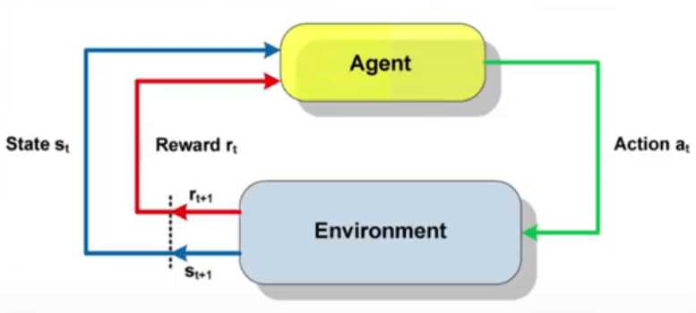
Reinforcement learning is a trial and error process where an AI (agent)
performs a number of actions in an environment. Each unique moment the
agent has a state and acts from this given state to a new one. This
particular action may on may not has a reward. Therefore, we can say that
each learning epoch (or an episode) can be represented as a sequence of states,
actions, and rewards. Each state depends only on the previous states and actions
and as the environment is inherently stochastic (we don’t know the state that
comes next), this process satisfies the Markov
property. The Markov property
says that the conditional probability distribution of future states of the
process depends only upon the present state, not on the sequence of events that
preceded it. The whole process is referred to as a Markov Decision
Process.
Let’s see a real example using Super Mario. In this case:
-
The agent is, of course, the beloved Mario
-
The state is the current situation (let’s say the frame of our screen)
-
The actions are: left, right movement and jump
-
The environment is the virtual world of each level;
-
And the reward is whether Mario is alive or dead.
Ok, we have properly defined the problem. What’s next? We need a solution. But
first, we need a way to evaluate how good the solution is?
What I am saying is that the reward on each episode it’s not enough. Imagine a
Mario game where the Mario is controlled by an agent. He is receiving constantly
positive rewards through the whole level by just before the final flag, he is
killed by one Hammer Bro (I hate those guys). You see that each individual
reward is not enough for us to win the game. We need a reward that captures the
whole level. This is where the term of the discounted cumulative expected
reward comes into play.
It is nothing more than the sum of all rewards discounted by a factor gamma,
where gamma belongs to [0,1). The discount is essential because the rewards tend
to be much more significant in the beginning than in the end. And it makes
perfect sense.
The next step is to solve the problem. To do that we define that the goal of the
learning task is: The agent needs to learn which action to perform from a given
state that maximized the cumulative reward over time. Or to learn the Policy
π: S->A. The policy is just a mapping between a state and an action.
To sum all the above, we use the following equation:
, where V (Value) is the expected long-term reward achieved by a policy
(π) from a state (s).
You still with me? If you are, let’s pause for 5 seconds cause this was a bit
overwhelming:
1…2…3…4…5
Now that we regain our mental clarity, let recap. We have the definition of the
problem as a Markov Decision Process and we have our goal to learn the best
Policy or the best Value. How we proceed?
We need an algorithm (Thank you, Sherlock…)
Well, there is an abundance of developed RL algorithms over the years. Each
algorithm focuses on a different thing, whether it is to maximize the value or
the policy or both. Whether to use a model(e.g a neural network) to simulate the
environment or not. Whether it will capture the reward on each step or the end.
As you guessed, it is not very easy to categorize all those algorithms in
classes, but that’s what I am about to do.
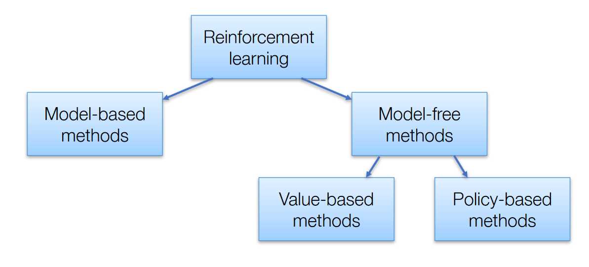
As you can see we can classify RL algorithms in two big categories: Model-based
and Model-free:
Model-based
These algorithms aim to learn how the environment works (its dynamics) from its
observations and then plan a solution using that model. When they have a model,
they use some planning method to find the best policy. They known to be data
efficient, but they fail when the state space is too large. Try to build a
model-based algorithm to play Go. Not gonna happen.
Dynamic programming methods
are an example of model-based methods, as they require the complete knowledge of
the environment, such as transition probabilities and rewards.
Model-free
Model-free algorithms do not require to learn the environment and store all the
combination of states and actions. The can be divided into two categories, based
on the ultimate goal of the training.
Policy-based methods try to find the optimal policy, whether it’s stochastic
or deterministic. Algorithms like policy gradients and REINFORCE belong in this
category. Their advantages are better convergence and effectiveness on high
dimensional or continuous action spaces.
Policy-based methods are essentially an optimization problem, where we find the
maximum of a policy function. That’s why we also use algorithms like evolution
strategies and hill climbing.
Value-based methods, on the other hand, try to find the optimal value. A big
part of this category is a family of algorithms called
Q-learning, which learn to optimize
the Q-Value. I plan to analyze Q-learning thoroughly on a next article because
it is an essential aspect of Reinforcement learning. Other algorithms involve
SARSA and value iteration.
At the intersection of policy and value-based method, we find the
Actor-Critic methods, where the goal is to optimize both the policy and the
value function.
And now to the cool part. In the past few years, there is a new kid in town. And
it was inevitable to affect and enhance all the existing methods to solve
Reinforcement Learning. I am sure you guessed it. Deep Learning. And thus, we
have a new term to represent all those new research ideas.
Deep Reinforcement Learning
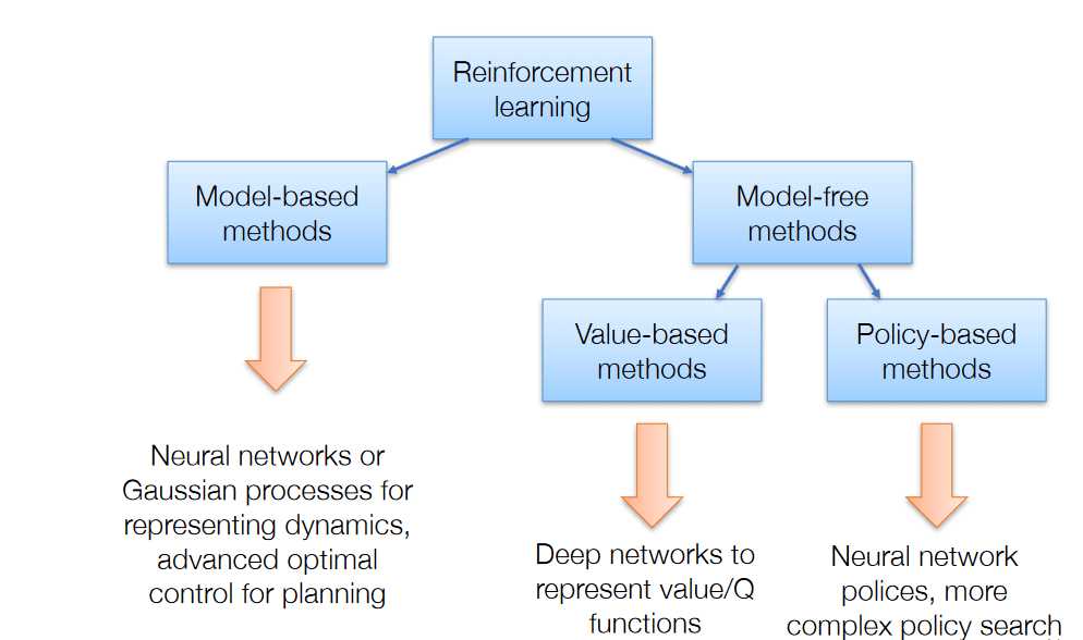
Deep neural networks have been used to model the dynamics of the
environment(mode-based), to enhance policy searches (policy-based) and to
approximate the Value function (value-based). Research on the last one (which is
my favorite) has produced a model called Deep Q
Network, which is responsible ,along with
its many improvements, for some of the most astonishing breakthroughs around the
area (take Atari for example). And to excite you, even more, we don’t just use
simple Neural Networks but Convolutional,
Recurrent and many else as well.
Ok, I think that’s enough for the first contact with Reinforcement Learning. I
just wanted to give you the basis behind the whole idea and present you an
overview of all the important techniques implemented over the years. But also,
to give you a hint of what’s next for the field. You want to explore more? Well first
that’s awesome. Second you can do so using this amazing set of courses by Coursera
Until my next article, stay tuned.
For the next article in the Reinforcement Learning Journey, click here.
* Disclosure: Please note that some of the links above might be affiliate links, and at no additional cost to you, we will earn a commission if you decide to make a purchase after clicking through.


