The journey to Reinforcement learning continues… It’s time to analyze the
infamous Q-learning and see how it became the new standard in the field of AI
(with a little help from neural networks).
First things first. In the last post , we saw the basic concept
behind Reinforcement Learning and we frame the problem using an agent, an
environment, a state (S), an action(A) and a reward (R). We talked about how the
whole process can be described as a Markov Decision Process and we introduced
the terms Policy and Value. Lastly, we had a quick high-level overview of the
basic methods out there.
Remember that the goal is to find the optimal policy and that policy is a
mapping between state and actions. So, we need to find which action to take
while we stand in a specific state in order to maximize our expected reward. One
way to find the optimal policy is to make use of the value functions (a
model-free technique).
And here we will get to the new stuff. In fact, there are two value functions
that are used today. The state value function V(s) and the action value function
Q(s, a) .
-
State value function: Is the expected return achieved when acting from a
state according to the policy. -
Action value function: Is the expected return given the state and the
action.
What is the difference you may ask? The first value is the value of a particular
state. The second one is the value of that state plus the values of all the
possible actions from that state.
When we have the action value function, the Q value, we can simply choose to
perform the action with the highest value from a state. But how do we find the Q
value?.
What is Q learning?
So, we will learn the Q value from trial and error? Exactly. We initialize the
Q, we choose an action and perform it, we evaluate it by measuring the reward
and we update the Q accordingly. In first, randomness will be a key player but
as the agent explores the environment, the algorithm will find the best Q value
for each state and action. Can we describe this mathematically?
Thank you Richard E. Bellmann. The above equation is known as the Bellman
equation and plays a huge part in RL today’s research. But what does it state?
The Q value, aka the maximum future reward for a state and action, is the
immediate reward plus the maximum future reward for the next state. And if you
think about it, it makes perfect sense. Gamma (γ) is a number between [0,1] and
its used to discount the reward as the time passes, given the assumption that
action in the beginning, are more important than at the end (an assumption that
is confirmed by many real-life use cases). As a result, we can update the Q
value iteratively.
The basic concept to understand here is that the Bellman equation relates
states with each other and thus, it relates Action value functions. That helps
us iterate over the environment and compute the optimal Values, which in turn
give us the optimal Policy.
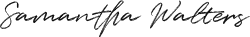
In its simplest form, Q values is a matrix with states as rows and actions as
columns. We initialize the Q-matrix randomly, the agent starts to interact with
the environment and measures the reward for each action. It then computes the
observed Q values and updates the matrix.
env = gym.make('MountainCar-v0')
Q = np.zeros([env.observation_space.n,env.action_space.n])
for i in range(episodes):
s = env.reset()
reward = 0
goal_flag = False
for j in range(200):
a = np.argmax(Q[s,:] + np.random.randn(1,env.action_space.n)*(1./(i+1)))
s_new,r,goal_flag,_ = env.step(a)
maxQ=np.max(Q[s_new,:])
Q[s,a] += lr*(r + g*maxQ - Q[s,a])
reward += r
s = s_new
if goal_flag == True:
break
Exploration vs Exploitation
The algorithm, as described above, is a greedy algorithm, as it always chooses the
action with the best value. But what if some action has a very small probability
to produce a very large reward? The agent will never get there. This is fixed by
adding random exploration. Every once in a while, the agent will perform a
random move, without considering the optimal policy. But because we want the
algorithm to converge at some point, we lower the probability to take a random
action as the game proceeds.
Why going Deep?
Q learning is good. No one can deny that. But the fact that it is ineffective in
big state spaces remains. Imagine a game with 1000 states and 1000 actions per
state. We would need a table of 1 million cells. And that is a very small state
space comparing to chess or Go. Also, Q learning can’t be used in unknown states
because it can’t infer the Q value of new states from the previous ones.
What if we approximate the Q values using some machine learning model. What if
we approximate them using neural networks? That simple idea (and execution of
course) was the reason behind DeepMind acquisition from Google for 500 million
dollars. DeepMind proposed an algorithm named Deep Q Learner and used it to play
Atari games with impeccable mastery.
Deep Q Learning
In deep Q learning, we utilize a neural network to approximate the Q value
function. The network receives the state as an input (whether is the frame of
the current state or a single value) and outputs the Q values for all possible
actions. The biggest output is our next action. We can see that we are not
constrained to Fully Connected Neural Networks, but we can use Convolutional,
Recurrent and whatever else type of model suits our needs.

I think it’s time to use all that stuff in practice and teach the agent play
Mountain Car. The goal is to make
a car drive up a hill. The car’s engine is not strong enough to climb the hill
in a single pass. Therefore, the only way to succeed is to drive back and forth
to build up momentum.

I will explain more about Deep Q Networks alongside with the code. First we should
build our Agent as a Neural Network with 3 Dense layers and we are goint to train it
using Adam optimization.
class DQNAgent:
def __init__(self, state_size, action_size):
self.state_size = state_size
self.action_size = action_size
self.memory = deque(maxlen=2000)
self.gamma = 0.95
self.epsilon = 1.0
self.epsilon_min = 0.01
self.epsilon_decay = 0.995
self.learning_rate = 0.001
self.model = self._build_model()
def _build_model(self):
model = Sequential()
model.add(Dense(24, input_dim=self.state_size, activation='relu'))
model.add(Dense(24, activation='relu'))
model.add(Dense(self.action_size, activation='linear'))
model.compile(loss='mse',
optimizer=Adam(lr=self.learning_rate))
return model
def remember(self, state, action, reward, next_state, done):
self.memory.append((state, action, reward, next_state, done))
def act(self, state):
if np.random.rand() <= self.epsilon:
return random.randrange(self.action_size)
act_values = self.model.predict(state)
return np.argmax(act_values[0])
Keypoints:
-
The agent holds a memory buffer with all past experiences.
-
His next action is determined by the maximum output (Q-value) of the network.
-
The loss function is the mean squared error of the predicted Q value and the target Q-value.
-
From the Bellman equation we have that the target is R + g*max(Q).
-
The difference between the target and the predicted values is called Temporal Difference Error (TD Error)
Before we train our DQN, we need to address an issue that plays a vital role on how the agent learns to estimate Q Values and this is:
Experience Replay
Experience replay is a concept where we help the agent to remember and not forget its previous actions by replaying them. Every once in a while, we sample a batch of previous experiences (which are stored in a buffer) and we feed the network. That way the agent relives its past and improve its memory. Another reason for this task is to force the agent to release himself from oscillation, which occurs due to high correlation between some states and resulting in the same actions over and over.
def replay(self, batch_size):
minibatch = random.sample(self.memory, batch_size)
for state, action, reward, next_state, done in minibatch:
target = reward
if not done:
Q_next=self.model.predict(next_state)[0]
target = (reward + self.gamma *np.amax(Q_next))
target_f = self.model.predict(state)
target_f[0][action] = target
self.model.fit(state, target_f, epochs=1, verbose=0)
Finally we get make our agent interact with the environment and train him
to predict the Q values for each next action
env = gym.make('MountainCar-v0')
state_size = env.observation_space.shape[0]
action_size = env.action_space.n
agent = DQNAgent(state_size, action_size)
done = False
batch_size = 32
for e in range(EPISODES):
state = env.reset()
state = np.reshape(state, [1, state_size])
for time in range(500):
action = agent.act(state)
next_state, reward, done, _ = env.step(action)
reward = reward if not done else -10
next_state = np.reshape(next_state, [1, state_size])
agent.remember(state, action, reward, next_state, done)
state = next_state
if done:
print("episode: {}/{}, score: {}, e: {:.2}"
.format(e, EPISODES, time, agent.epsilon))
break
if len(agent.memory) > batch_size:
agent.replay(batch_size)
As you can see is the exact same process with the Q-table example, with the difference
that the next action comes by the DQN prediction and not by the Q-table. As a result,
it can be applied to unknown states. That’s the magic of Neural Networks.
You just created an agent that learns to drive the car up the hill. Awesome. And what is
more awesome is that the exact same code(i mean copy paste) can be used in many more games,
from Atari and Super Mario to Doom(!!!)
Awesome!
Just on more time, I promise.
Awesome!
If you need extra material, I can’t recommend enough the Advanced AI: Deep Reinforcement Learning Course in Python on Udemy. It covers everything you will need on Deep Q Learning and much much more.
In the next episode, we will remain on the Deep Q Learning area and discuss some more advanced
techniques such as Double DQN Networks, Dueling DQN and Priotitized Experience replay.
See you soon…

* Disclosure: Please note that some of the links above might be affiliate links, and at no additional cost to you, we will earn a commission if you decide to make a purchase after clicking through.