Hello again,
Today’s topic is … well, the same as the last one. Q Learning and Deep Q
Networks. Last time, we explained what Q Learning is and how to use the Bellman
equation to find the Q-values and as a result the optimal policy. Later, we
introduced Deep Q Networks and how instead of computing all the values of the
Q-table, we let a Deep Neural Network learn to approximate them.
Deep Q Networks take as input the state of the environment and output a Q value
for each possible action. The maximum Q value determines, which action the agent
will perform. The training of the agents uses as loss the TD Error, which is
the difference between the maximum possible value for the next state and the
current prediction of the Q-value (as the Bellman equation suggests). As a
result, we manage to approximate the Q-tables using a Neural Network.
So far so good. But of course, there are a few problems that arise. It’s just
the way scientific research is moving forward. And of course, we have come up
with some great solutions.
Moving Q-Targets
The first problem is what is called moving Q-targets. As we saw, the first
component of the TD Error (TD stands for Temporal Difference) is the Q-Target
and it is calculated as the immediate reward plus the discounted max Q-value for
the next state. When we train our agent, we update the weights accordingly to
the TD Error. But the same weights apply to both the target and the predicted
value. You see the problem?
We move the output closer to the target, but we also move the target. So, we end
up chasing the target and we get a highly oscillated training process. Wouldn’t
be great to keep the target fixed as we train the network. Well, DeepMind did
exactly that.
Instead of using one Neural Network, it uses two. Yes, you heard that right!
(like one wasn’t enough already).
One as the main Deep Q Network and a second one (called Target Network) to
update exclusively and periodically the weights of the target. This technique is
called Fixed Q-Targets. In fact, the weights are fixed for the largest part
of the training and they updated only once in a while.
class DQNAgent:
def __init__(self, state_size, action_size):
self.model = self._build_model()
self.target_model = self._build_model()
self.update_target_model()
def update_target_model(self):
self.target_model.set_weights(self.model.get_weights())
Maximization Bias
Maximization bias is the tendency of Deep Q Networks to overestimate both the
value and the action-value (Q) functions. Why does it happen? Think that if for
some reason the network overestimates a Q value for an action, that action will
be chosen as the go-to action for the next step and the same overestimated value
will be used as a target value. In other words, there is no way to evaluate if
the action with the max value is actually the best action. How to solve this?
The answer is a very interesting method and is called:
Double Deep Q Network
To address maximization bias, we use two Deep Q Networks.
-
On the one hand, the DQN is responsible for the selection of the next
action (the one with the maximum value) as always. -
On the other hand, the Target network is responsible for the evaluation
of that action.
The trick is that the target value is not automatically produced by the maximum
Q-value, but by the Target network. In other words, we call forth the Target
network to calculate the target Q value of taking that action at the next state.
And as a side effect, we also solve the moving target problem. Neat right? Two
birds with one stone. By decoupling the action selection from the target Q-value
generation, we are able to substantially reduce the overestimation, and train
faster and more reliably.
def train_model(self):
if len(self.memory) < self.train_start:
return
batch_size = min(self.batch_size, len(self.memory))
mini_batch = random.sample(self.memory, batch_size)
update_input = np.zeros((batch_size, self.state_size))
update_target = np.zeros((batch_size, self.state_size))
action, reward, done = [], [], []
for i in range(batch_size):
update_input[i] = mini_batch[i][0]
action.append(mini_batch[i][1])
reward.append(mini_batch[i][2])
update_target[i] = mini_batch[i][3]
done.append(mini_batch[i][4])
target = self.model.predict(update_input)
target_next = self.model.predict(update_target)
target_val = self.target_model.predict(update_target)
for i in range(self.batch_size):
if done[i]:
target[i][action[i]] = reward[i]
else:
a = np.argmax(target_next[i])
target[i][action[i]] = reward[i] + self.discount_factor * (target_val[i][a])
self.model.fit(update_input, target, batch_size=self.batch_size,epochs=1, verbose=0)
You think that’s it? Sorry to let you down. We are going to take this even
further. What now? Are you going to add a third Neural Network? Haha!!
Well kind of. Who’s laughing now?
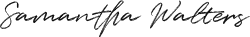
Dueling Deep Q Networks
Let’s refresh the basis of Q Learning first. Q values correspond to a metric of
how good an action is for a particular state right? That’s why it is an
action-value function. The metric is nothing more the expected return of that
action from the state. Q values can, in fact, be decomposed into two pieces: the
state Value function V(s) and the advantage value A(s, a). And yes, we just
introduce one more function:
Advantage function captures how better an action is compared to the others at a
given state, while as we know the value function captures how good it is to be
at this state. The whole idea behind Dueling Q Networks relies on the
representation of the Q function as a sum of the Value and the advantage
function. We simply have two networks to learn each part of the sum and then
we aggregate their outputs.

Dueling Network Architectures for Deep Reinforcement Learning
Do we earn something by doing that? Of course, we do. The agents in now able to
evaluate a state without caring about the effect of each action from that state.
Meaning that the features that determined whether a state is good or nor are not
necessarily the same as the features that evaluate an action. And it may not
need to care for actions at all. It is not uncommon to have actions from a state
that do not affect the environment at all. So why take them into consideration?
* Quick note: If you take a closer look at the image, you will see that to
aggregate the output of the two networks we do not simply add them. The reason
behind that is the issue of identifiability. If we have the Q, we can’t find the
V and A. So, we can’t back propagate. Instead, we choose to use the mean
advantage as a baseline (the subtracted term).
def build_model(self):
input = Input(shape=self.state_size)
shared = Conv2D(32, (8, 8), strides=(4, 4), activation='relu')(input)
shared = Conv2D(64, (4, 4), strides=(2, 2), activation='relu')(shared)
shared = Conv2D(64, (3, 3), strides=(1, 1), activation='relu')(shared)
flatten = Flatten()(shared)
advantage_fc = Dense(512, activation='relu')(flatten)
advantage = Dense(self.action_size)(advantage_fc)
advantage = Lambda(lambda a: a[:, :] - K.mean(a[:, :], keepdims=True),
output_shape=(self.action_size,))(advantage)
value_fc = Dense(512, activation='relu')(flatten)
value = Dense(1)(value_fc)
value = Lambda(lambda s: K.expand_dims(s[:, 0], -1),
output_shape=(self.action_size,))(value)
q_value = merge([value, advantage], mode='sum')
model = Model(inputs=input, outputs=q_value)
model.summary()
return model
Last but not least, we have on more issue to discuss and it has to do with
optimizing the experience replay.
Prioritized Experience Replay
Do you remember that experience replay is when we replay to the agent random
past experiences every now and then to prevent him from forgetting them? If you
don’t, now you do. But some experiences may be more significant than others. As
a result, we should prioritize them to be replayed. To do just that, instead of
sampling randomly (from a uniform distribution), we sample using a priority. As
priority we define the magnitude of the TD Error (plus some constant to avoid
zero probability for an experience to be chosen).
Central idea: The highest the error between the prediction and the target, the
more urgent is to learn about it.
And to ensure that we won’t always replay the same experience, we add some
stochasticity and we are all set. Also, for complexity’s shake we save the experiences in
a binary tree called SumTree.
from SumTree import SumTree
class PER:
e = 0.01
a = 0.6
def __init__(self, capacity):
self.tree = SumTree(capacity)
def _getPriority(self, error):
return (error + self.e) ** self.a
def add(self, error, sample):
p = self._getPriority(error)
self.tree.add(p, sample)
def sample(self, n):
batch = []
segment = self.tree.total() / n
for i in range(n):
a = segment * i
b = segment * (i + 1)
s = random.uniform(a, b)
(idx, p, data) = self.tree.get(s)
batch.append((idx, data))
return batch
def update(self, idx, error):
p = self._getPriority(error)
self.tree.update(idx, p)
That was a lot. A lot of new information, a lot of new improvements. But just
think what we can combine all of them together. And we do it.
I tried to give a summary of the most important recent efforts in the field,
backed by some intuitive thought and some math. This is why Reinforcement
Learning is so important to learn. There is so much potential and so many
capabilities for enhancements that you just can’t ignore the fact that is going
to be the big player in AI (if it already isn’t). But that’s why is so hard to
learn and to keep up with it.
If you need to dive deeper, I highly suggest the Advanced AI: Deep Reinforcement Learning Course in Python on Udemy.
Next time, we will introduce Policy Gradients and the REINFORCE algorithm
All we have to do is keep learning …

* Disclosure: Please note that some of the links above might be affiliate links, and at no additional cost to you, we will earn a commission if you decide to make a purchase after clicking through.